In this post, we will build a CART Decision Tree model in Python from scratch. We will start with the foundational principals, and work straight through to implementation in code. Both classification and regression examples will be included.
Table of Contents
Note: for those who prefer video content, you can watch me work through the content in this article by scrolling to the bottom of this post.
Motivation to Build a Decision Tree Model
Decision Trees are a family of non-parametric1 supervised learning models that are based upon simple boolean decision rules to predict an outcome. The space defined by the independent variables \bold{X} is termed the feature space. Decision Trees split the feature space according to decision rules, and this partitioning is continued until some stopping criteria is met. In practice, this process typically achieved through recursion. A simple statistic, such as the mean, median, or mode, can then be calculated on the data contained in each of the final partitions. This statistic can serve as an estimate for the label \bold{y}. Decision Trees can be applied to both classification and regression problems, and constitute some of the most popular machine learning algorithms used in industry.
There are a wide variety of Decision Tree algorithms available. Some notable examples include:
- Chi-square Automatic Interaction Detection (CHAID) – developed by Gordon V. Kass in 19802
- Classification And Regression Tree (CART) – invented by Leo et al. in 19843
- Iterative Dichotomiser 3 (ID3) – invented by Ross Quinlan in 19864
- C4.5 – invented by Ross Quinlan in 19935 as an extension of the ID3 algorithm
In this article, we will focus on CART. The main advantages of this approach include:
- Simplicity of the model, which facilitates interpretability. Output of the model can be easily explained by the decision rules. The model can be visualised in an intuitive fashion.
- Minimal data preparation is required. Whereas other algorithms may require the data to be normalised, the creation of dummy variables, accounting for missing/NaN values, etc., these steps aren’t required for Decision Trees.
The primary disadvantages include:
- Instability due to small variations in the dataset. This can lead to completely different trees being generated.
- Practical tree learning algorithms use a heuristic approach (i.e. the ‘greedy algorithm’) that cannot guarantee a globally optimal solution.
It should be noted that both disadvantages listed above are normally addressed through the use of ensembles. See my articles on Bagging, Random Forest, Adaboost Classification, Adaboost Regression, and Gradient Boost for examples of ensembles.
Assumptions and Considerations to Build a Decision Tree Model
Like other non-parametric models, Decision Trees do not rely on any assumptions regarding the distributions in the underlying data. However, there are a number of aspects to this algorithm that should be considered regarding their practical application:
- Depending on the implementation, missing or NaN values may need to be accounted for.
- Decision trees tend to overfit in situations where the dataset has a very large number of features. Truncating the number of features, by applying a dimensionality reduction algorithm as a preprocessing step, may enhance performance.
- Decision Trees tend to be biased in situations where certain classes have a higher frequency in the dataset. The dataset should be balanced6 prior to training.
Derivation of Decision Trees
Decision Trees are comprised of a set of connected nodes where binary decisions are made to define how the data are split. Data can be pictured as ‘flowing’ through the tree, passing from node to node, until a final partition of the data is arrived at. The node from which data flows from can be termed the parent, while the node to which data flows to is the child. There are 3 types of nodes:
- Root node: this is where all the data starts and where the initial decision rule is applied. This node has no parent.
- Interior nodes: these are the locations where decision rules are applied on the data that are passed from the parent. The resulting partitioned data are then passed to the children.
- Leaf nodes: these nodes define the final partition of the data, and determine the ultimate output of the model. These nodes have no children.
We can illustrate this structure with a simple toy example. Let’s construct a tree for determining whether a vertebrate animal is a mammal or bird:
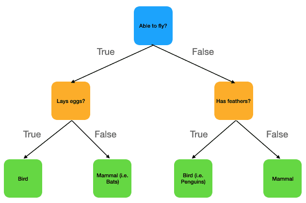
This figure outlines a simple Decision Tree for distinguishing between mammals and birds. This is based off of 3 decision rules:
- Ability to fly?
- Lays eggs?
- Has feathers?
The nodes are colour coded:
- Root node: blue
- Interior nodes: orange
- Leaf nodes: green
Data that pass the decision rule at any given node flow to the left child, otherwise the data flow to the right child. Notice that this tree has two layers of depth.
To make our discussion more concrete, let’s run through the CART algorithm procedure for growing/training a Decision Tree. This includes:
- Select a metric upon which the decision rules will be based.
- Start at the root node with all the training data.
- Choose one feature, and threshold value, by which the training data will be split that minimises our metric. Record the feature – threshold value pair.
- Partition the data according to the chosen feature and threshold, then repeat steps 3 and 4 for each subset of the data.
- Stop partitioning when: i) all samples in the given node have the same label \bold{y}, ii) a specified model limit is reached (e.g. maximum tree depth, etc.). In the terminal partitions, compute the leaf node values, and record these.
Once we have a trained Decision Tree, generating predictions on unseen data is straightforward. We can pass the data through the tree, starting at the root node, and move to either the left or right child node. The choice of moving right or left depends on how these data satisfy the decision rules (which are based on the feature – threshold pairs stored in step 3 above). We navigate through the tree in this manner until a leaf node is reached. At this point, the stored leaf node value is provided as the prediction.
The metric we choose in step 1 above will depend on the type of problem we are trying to solve. What we want is to measure the information content of each feature in the dataset: more informative features tell us more about a problem than less informative features. At any given node, we choose the most informative feature to split on, along with an optimised split value. The metrics we use in this step are termed impurity metrics.
Say our training data is comprised of independent \bold{X} and dependent \bold{y} variables:
\bold{y} = \begin{bmatrix} y_1 \\ y_2 \\ . \\ . \\ . \\ y_N \end{bmatrix}, \bold{X} = \begin{bmatrix} x_{1,1} & x_{1,2} & … & x_{1,M} \\ x_{2,1} & x_{2,2} & … & x_{2,M} \\ … & … & … & … \\ … & … & … & … \\ x_{N,1} & x_{N,2} & … & x_{N,M} \end{bmatrix} (1)
There are M features in this dataset, along with a total of N samples. The feature set is defined by the column vectors \{ \bold{x}_f \} that make up \bold{X}, where f = 1..M. The goal of splitting the data set is to find the feature f^*, and threshold value x_{f^*} for this feature, such that the impurity metric is minimised.
Let’s define the total data matrix as the combination of \bold{X} and \bold{y}:
\bold{D} = \begin{bmatrix} x_{1,1} & x_{1,2} & … & x_{1,M} & y_1 \\ x_{2,1} & x_{2,2} & … & x_{2,M} & y_2 \\ … & … & … & … & … \\ … & … & … & … & … \\ x_{N,1} & x_{N,2} & … & x_{N,M} & y_N \end{bmatrix} (2)
The splitting procedure can then be written as:
\bold{D}_{left} = \bold{D}|\bold{x}_{f^*} \le x_{f^*} (3a)
\bold{D}_{right} = \bold{D}|\bold{x}_{f^*} > x_{f^*} (3b)
where it is understood that the inequalities in (3) are done element-wise over \bold{x}_f. The impurity for this split is measured using the chosen impurity metric I_p:
I_p^{node} = \frac{N_{left}}{N_{node}}I_p(\bold{D}_{left}) + \frac{N_{right}}{N_{node}}I_p(\bold{D}_{right}) (4)
where N_{left} is the number of samples that satisfy (3a), and N_{right} is the number of samples that satisfy (3b). N_{node} is the total number of samples being considered. The calculation of (4) is repeated over all possible feature and split values, to determine the lowest possible I_p^{node}:
\{ f^*,x_{f^*} \} = argmin_{ \{ f,x_f \} }I_p^{node} (5)
Note that the approach outlined through (3), (4), and (5) is a greedy algorithm, in that it makes locally optimal choices for the feature and split values. This cannot guarantee a globally optimal solution, but in practice this is the most computationally expedient option, and is most widely used in practice. These equations can be executed in a recursive manner to grow the tree until our stopping criteria are met.
Our choice of I_p will depend upon whether we are dealing with a classification or regression problem. In regression trees, the label \bold{y} can take on continuous values, whereas for classification trees only discrete values are permitted.
Let’s start with classification: we can begin by defining the proportion of class c at the current node:
p_c^{node} = \frac{1}{N_{node}} \sum_{i=1.. N_{node}} \bold{I}(y_i = c) (6)
where \bold{I} is the identity function and i is the index over all samples at the current node. A common impurity metric for classification is the gini impurity:
I_p(\bold{D}_{node}) = \sum_c p_c^{node}(1 – p_c^{node}) (7)
Intuitively, the gini impurity is a measure of the probability of misclassifying a datapoint at the given node. The lowest possible value is 0, which indicates a perfect fit to the data.
Alternatively, we could use the Shannon entropy:
I_p(\bold{D}_{node}) = -\sum_c p_c^{node}\log_2(p_c^{node}) (8)
The intuition behind this quantity is that it yields a measure of the information content contained within the data provided. Situations where the data contains a near-equal distribution among all possible classes c will have high entropy, whereas data with almost all samples belonging to one class will have very low entropy. The lowest possible value is also 0, indicating a completely deterministic process.
For the case of regression, let’s start with computing the the mean of the label values \bold{y}:
y^{node} = \frac{1}{N_{node}}\sum_{i=1.. N_{node}}y_i (9)
We can then compute the mean squared error (MSE) of each sample label in the node with respect to (9):
I_p(\bold{D}_{node}) = \frac{1}{N_{node}}\sum_{i =1 .. N_{node}}(y_i – y^{node})^2 (10)
The mean squared error gives more weight to outliers that are present in the data. The lowest possible value is 0, indicating all labels in the node have the same value.
The impurity can also be measured through the mean absolute error (MAE) of each sample label in the node with respect to (9):
I_p(\bold{D}_{node}) = \frac{1}{N_{node}}\sum_{i =1 .. N_{node}}|y_i – y^{node}| (11)
This metric is easier to understand than (10): it is the average deviation between the sample labels and (9). Like the case of the mean squared error, the lowest possible value is 0, indicating all labels in the node have the same value.
Note that (9) can be replaced with other measures of the average label value at the node, most notably the median. The median is more robust against the presence of outliers in the data, and as such could help improve performance.
Build and Test Decision Trees in Python
We’ll now work through an implementation of both classification and regression Decision Trees in Python. For the classification problem, I will make use of the same breast cancer dataset that was already examined in the Logistic Regression post. As such, I will not do a detailed exploration of these data in this article.
Build a Decision Tree Model
First, I will import all the packages required:
# imports
from __future__ import annotations
from typing import Tuple
from abc import ABC,abstractmethod
from scipy import stats
import numpy as np
import pandas as pd
import matplotlib.pyplot as plt
from sklearn.model_selection import train_test_split
from sklearn.datasets import load_breast_cancer,make_regression
from sklearn.metrics import accuracy_score,precision_score,recall_score,mean_squared_error,mean_absolute_error,r2_score
Next I will build a class that defines the functionality of each node in our tree:
class Node(object):
    """
    Class to define & control tree nodes
    """

    def __init__(self) -> None:
        """
        Initializer for a Node class instance
        """
        self.__split    = None
        self.__feature  = None
        self.__left     = None
        self.__right    = None
        self.leaf_value = None

    def set_params(self, split: float, feature: int) -> None:
        """
        Set the split & feature parameters for this node

        Input:
            split   -> value to split feature on
            feature -> index of feature to be used in splitting
        """
        self.__split   = split
        self.__feature = feature

    def get_params(self) -> Tuple[float,int]:
        """
        Get the split & feature parameters for this node

        Output:
            Tuple containing (split,feature) pair
        """
        return(self.__split, self.__feature)

    def set_children(self, left: Node, right: Node) -> None:
        """
        Set the left/right child nodes for the current node

        Inputs:
            left  -> LHS child node
            right -> RHS child node
        """
        self.__left  = left
        self.__right = right

    def get_left_node(self) -> Node:
        """
        Get the left child node

        Output:
            LHS child node
        """
        return(self.__left)

    def get_right_node(self) -> Node:
        """
        Get the RHS child node

        Output:
            RHS child node
        """
        return(self.__right)
The Node class member functions are as follows:
- __init__(self) : this is the initialiser function which executes automatically when a class instance is declared. The model parameters are initialised here.
- set_params(self, split, feature) : this function is used to set values to the split parameters (threshold x_{f^*} and feature f^*) for this node.
- get_params(self) : this function returns the split parameters (threshold x_{f^*} and feature f^*) for this node.
- set_children(self, left, right): this function assigns child nodes to the current node. Input arguments left and right are also assumed to be of type Node.
- get_left_node(self) : return the left child node.
- get_right_node(self) : return the right child node.
We will now proceed to define classes that will be used to build our trees. Since both regression and classification trees are structurally similar, where the key differences are in terms of the impurity metrics and how the leaf node values are calculated, I will take an object-oriented (OO) approach to avoid writing duplicate code. This will consist of writing:
- one class for all the functionality common to both the classification and regression use cases.
- one class for all the functionality unique to the classification use case.
- one class for all the functionality unique to the regression use case.
This construction will make use of inheritance, where one class can take on the attributes of another class. Specifically, class 1 mentioned above will serve as our base class, which will consist of all the functionality and data that are common between classes 2 and 3. Classes 2 and 3 will inherit from class 1, and are termed the child classes.
Notice how class 1 only serves as a repository of common functionality and data between the classification and regression child classes. We will never need to create an instance of class 1, instead we only want to use it while building classes 2 & 3. As such, class 1 will be set up as an abstract class: these are classes with incomplete definitions that are solely used as a basis for inheritance in child classes. Abstract classes also allow for the definition of a common API among all child classes. It is not possible to create an instance of an abstract class.
Proceeding with the OO approach, for all the classes built in this article I will follow the public, protected, and private convention for accessing resources:
- public member variables and functions of a class are accessible everywhere, both within and outside the class. In the Node class above, all member functions except for __init__ are public, whereas only the leafv member variable is public.
- protected member variables and functions of a class are accessible within the class, and to any inherited daughter classes. These will be indicated by a single underscore, ‘_’ at the start of the member name. The Node class does not have any protected members.
- private member variables and functions of a class are only accessible within the class where they are declared. These will be indicated by a double underscore, ‘__’ at the start of the member name. In the Node class, only the __init__ member function is private, whereas all the member variables except leafv are private.
It is important to note that unlike C++ or Java, Python does not enforce this access convention. As such it is up to the engineer to ensure this is being followed in the code.
We’ll start defining our abstract base class, DecisionTree. Let’s take a look at how to implement this class:
class DecisionTree(ABC):
    """
    Base class to encompass the CART algorithm
    """

    def __init__(self, max_depth: int=None, min_samples_split: int=2) -> None:
        """
        Initializer

        Inputs:
            max_depth         -> maximum depth the tree can grow
            min_samples_split -> minimum number of samples required to split a node
        """
        self.tree              = None
        self.max_depth         = max_depth
        self.min_samples_split = min_samples_split
In Python, abstract base classes require the ABC module is passed as an argument. The initialiser includes two hyper parameters for the model:
- max_depth : this defines the maximum number of levels to be allowed while growing the tree (default None).
- min_samples_split : this defines the minimum number of samples to allow a split to occur at any given node (default 2).
Both of these hyper parameters act to prevent the tree from overfitting on the training data, and should be determined through cross-validation on the dataset.
Next, we will look at the member functions that cover the impurity metric and leaf node value:
    @abstractmethod
    def _impurity(self, D: np.array) -> None:
        """
        Protected function to define the impurity
        """
        pass

    @abstractmethod
    def _leaf_value(self, D: np.array) -> None:
        """
        Protected function to compute the value at a leaf node
        """
        pass
Notice that both functions lack a definition, and both have the @abstractmethod decorator. This decorator indicates that these are abstract methods; these are methods which will be defined later in the child class that inherits from DecisionTree. What is established here is the API to both of these functions; both will take in a data matrix D and return the impurity metric or leaf value, respectively.
We will now look at the private recursive function used to grow the tree during training:
    def __grow(self, node: Node, D: np.array, level: int) -> None:
        """
        Private recursive function to grow the tree during training

        Inputs:
            node  -> input tree node
            D     -> sample of data at node
            level -> depth level in the tree for node
        """
        # are we in a leaf node?
        depth = (self.max_depth is None) or (self.max_depth >= (level+1))
        msamp = (self.min_samples_split <= D.shape[0])
        n_cls = np.unique(D[:,-1]).shape[0] != 1

        # not a leaf node
        if depth and msamp and n_cls:

            # initialize the function parameters
            ip_node = None
            feature = None
            split   = None
            left_D  = None
            right_D = None
            # iterate through the possible feature/split combinations
            for f in range(D.shape[1]-1):
                for s in np.unique(D[:,f]):
                    # for the current (f,s) combination, split the dataset
                    D_l = D[D[:,f]<=s]
                    D_r = D[D[:,f]>s]
                    # ensure we have non-empty arrays
                    if D_l.size and D_r.size:
                        # calculate the impurity
                        ip  = (D_l.shape[0]/D.shape[0])*self._impurity(D_l) + (D_r.shape[0]/D.shape[0])*self._impurity(D_r)
                        # now update the impurity and choice of (f,s)
                        if (ip_node is None) or (ip < ip_node):
                            ip_node = ip
                            feature = f
                            split   = s
                            left_D  = D_l
                            right_D = D_r
            # set the current node's parameters
            node.set_params(split,feature)
            # declare child nodes
            left_node  = Node()
            right_node = Node()
            node.set_children(left_node,right_node)
            # investigate child nodes
            self.__grow(node.get_left_node(),left_D,level+1)
            self.__grow(node.get_right_node(),right_D,level+1)

        # is a leaf node
        else:

            # set the node value & return
            node.leaf_value = self._leaf_value(D)
            return
The arguments to this function include an instance of Node, representing the current node in the tree, the associated data matrix \bold{D}_{node}, and an integer indicating the current level/depth in the tree. The function first checks if the current node is a leaf node:
- if not then every possible feature/split value combination is compared to determined the optimal \{ f^*,x_{f^*} \} pair. This comparison is done using the impurity metric selected for the problem in equation (4). Once an optimal split of the data matrix is determined, left and right child nodes are created, and then the function calls itself for each of the child nodes.
- if it is a leaf node, then the leaf value is determined and the function returns.
A second private recursive function is used to traverse a trained tree:
    def __traverse(self, node: Node, Xrow: np.array) -> int | float:
        """
        Private recursive function to traverse the (trained) tree

        Inputs:
            node -> current node in the tree
            Xrow -> data sample being considered
        Output:
            leaf value corresponding to Xrow
        """
        # check if we're in a leaf node?
        if node.leaf_value is None:
            # get parameters at the node
            (s,f) = node.get_params()
            # decide to go left or right?
            if (Xrow[f] <= s):
                return(self.__traverse(node.get_left_node(),Xrow))
            else:
                return(self.__traverse(node.get_right_node(),Xrow))
        else:
            # return the leaf value
            return(node.leaf_value)
This function is called while generating predictions with a trained tree. It takes two arguments besides self, an instance of Node that represents the current node in the tree, and a single sample of the independent variables represented by a row in \bold{X}. If the current node isn’t a leaf node, then the stored split parameters \{ f^*,x_{f^*} \} for the node is retrieved, and used to determine whether to go to the left or right child according to equation (3). If the current node is a leaf node, then the stored value is returned.
The last two member functions for this class are public, and are used to train the model and generate predictions:
    def train(self, Xin: np.array, Yin: np.array) -> None:
        """
        Train the CART model

        Inputs:
            Xin -> input set of predictor features
            Yin -> input set of labels
        """
        # prepare the input data
        D = np.concatenate((Xin,Yin.reshape(-1,1)),axis=1)
        # set the root node of the tree
        self.tree = Node()
        # build the tree
        self.__grow(self.tree,D,1)

    def predict(self, Xin: np.array) -> np.array:
        """
        Make predictions from the trained CART model

        Input:
            Xin -> input set of predictor features
        Output:
            array of prediction values
        """
        # iterate through the rows of Xin
        p = []
        for r in range(Xin.shape[0]):
            p.append(self.__traverse(self.tree,Xin[r,:]))
        # return predictions
        return(np.array(p).flatten())
Note that the input to the train member function has the independent and dependent variables separated, as is the form in equation (1). These arrays are combined into a single object, \bold{D}_{node}, according to equation (2), before creating the root node of the tree, and then making a call to __grow. The predict function only takes in the independent variables, and iterates through each row contained in the input to generate predictions.
We will now define the child class for classification problems, DecisionTreeClassifier:
class DecisionTreeClassifier(DecisionTree):
    """
    Decision Tree Classifier
    """

    def __init__(self, max_depth: int=None, min_samples_split: int=2, loss: str='gini') -> None:
        """
        Initializer

        Inputs:
            max_depth         -> maximum depth the tree can grow
            min_samples_split -> minimum number of samples required to split a node
            loss              -> loss function to use during training
        """
        DecisionTree.__init__(self,max_depth,min_samples_split)
        self.loss = loss

    def __gini(self, D: np.array) -> float:
        """
        Private function to define the gini impurity

        Input:
            D -> data to compute the gini impurity over
        Output:
            Gini impurity for D
        """
        # initialize the output
        G = 0
        # iterate through the unique classes
        for c in np.unique(D[:,-1]):
            # compute p for the current c
            p = D[D[:,-1]==c].shape[0]/D.shape[0]
            # compute term for the current c
            G += p*(1-p)
        # return gini impurity
        return(G)

    def __entropy(self, D: np.array) -> float:
        """
        Private function to define the shannon entropy

        Input:
            D -> data to compute the shannon entropy over
        Output:
            Shannon entropy for D
        """
        # initialize the output
        H = 0
        # iterate through the unique classes
        for c in np.unique(D[:,-1]):
            # compute p for the current c
            p = D[D[:,-1]==c].shape[0]/D.shape[0]
            # compute term for the current c
            H -= p*np.log2(p)
        # return entropy
        return(H)

    def _impurity(self, D: np.array) -> float:
        """
        Protected function to define the impurity

        Input:
            D -> data to compute the impurity metric over
        Output:
            Impurity metric for D
        """
        # use the selected loss function to calculate the node impurity
        ip = None
        if self.loss == 'gini':
            ip = self.__gini(D)
        elif self.loss == 'entropy':
            ip = self.__entropy(D)
        # return results
        return(ip)

    def _leaf_value(self, D: np.array) -> int:
        """
        Protected function to compute the value at a leaf node

        Input:
            D -> data to compute the leaf value
        Output:
            Mode of D
        """
        return(stats.mode(D[:,-1],keepdims=False)[0])
Note that DecisionTreeClassifier takes as an argument DecisionTree. In Python, this indicates that class DecisionTreeClassifier is a child class of DecisionTree. Let’s review the class member functions:
- __init__(self, max_depth, min_samples_split, loss) : this is the initialiser function which executes automatically when a class instance is declared. The initialiser for the base class is explicitly called as well. Model parameters are initialised here. An additional hyper parameter is included: loss, which can take on values ‘gini’ or ‘entropy’.
- __gini(self, D) : this private function is used to implement the gini impurity metric according to equation (7).
- __entropy(self, D) : this private function is used to implement the entropy impurity metric according to equation (8).
- _impurity(self, D): this protected function defines an implementation for the abstract method in the base class. The choice of impurity metric is made here.
- _leaf_value(self, D) : this protected function defines an implementation for the abstract method in the base class. Values for leaf nodes are determined here.
Finally, we will define the child class for regression problems, DecisionTreeRegressor:
class DecisionTreeRegressor(DecisionTree):
    """
    Decision Tree Regressor
    """

    def __init__(self, max_depth: int=None, min_samples_split: int=2, loss: str='mse') -> None:
        """
        Initializer

        Inputs:
            max_depth         -> maximum depth the tree can grow
            min_samples_split -> minimum number of samples required to split a node
            loss              -> loss function to use during training
        """
        DecisionTree.__init__(self,max_depth,min_samples_split)
        self.loss = loss

    def __mse(self, D: np.array) -> float:
        """
        Private function to define the mean squared error

        Input:
            D -> data to compute the MSE over
        Output:
            Mean squared error over D
        """
        # compute the mean target for the node
        y_m = np.mean(D[:,-1])
        # compute the mean squared error wrt the mean
        E = np.sum((D[:,-1] - y_m)**2)/D.shape[0]
        # return mse
        return(E)

    def __mae(self, D: np.array) -> float:
        """
        Private function to define the mean absolute error

        Input:
            D -> data to compute the MAE over
        Output:
            Mean absolute error over D
        """
        # compute the mean target for the node
        y_m = np.mean(D[:,-1])
        # compute the mean absolute error wrt the mean
        E = np.sum(np.abs(D[:,-1] - y_m))/D.shape[0]
        # return mae
        return(E)

    def _impurity(self, D: np.array) -> float:
        """
        Protected function to define the impurity

        Input:
            D -> data to compute the impurity metric over
        Output:
            Impurity metric for D
        """
        # use the selected loss function to calculate the node impurity
        ip = None
        if self.loss == 'mse':
            ip = self.__mse(D)
        elif self.loss == 'mae':
            ip = self.__mae(D)
        # return results
        return(ip)

    def _leaf_value(self, D: np.array) -> float:
        """
        Protected function to compute the value at a leaf node

        Input:
            D -> data to compute the leaf value
        Output:
            Mean of D
        """
        return(np.mean(D[:,-1]))
Let’s review the class member functions:
- __init__(self, max_depth, min_samples_split, loss) : this is the initialiser function which executes automatically when a class instance is declared. The initialiser for the base class is explicitly called as well. Model parameters are initialised here. An additional hyper parameter is included: loss, which can take on values ‘mse’ or ‘mae’.
- __mse(self, D) : this private function is used to implement the mean squared error impurity metric according to equation (10).
- __mae(self, D) : this private function is used to implement the mean absolute error impurity metric according to equation (11).
- _impurity(self, D): this protected function defines an implementation for the abstract method in the base class. The choice of impurity metric is made here.
- _leaf_value(self, D) : this protected function defines an implementation for the abstract method in the base class. Values for leaf nodes are determined here.
Important point: to make instances of a child class, all the abstract methods in the base class must have implementations. If this isn’t the case, the child class will also be an abstract base class.
Now that our tree models are implemented, let’s proceed to test out their performance. We’ll start with the classification Decision Tree. To do this, let’s load in the same breast cancer dataset used in the Logistic Regression post.
Classification Dataset Exploration
# load classification dataset
data = load_breast_cancer()
X    = data.data
y    = data.target
One question to ask at this point is whether this dataset is balanced or not? Let’s produce a simple histogram to address this question:
# is the dataset balanced?
plt.hist(y)
plt.xlabel('classes')
plt.ylabel('counts')
plt.show()
print('Percentage of y=0: ',y[y==0].shape[0]/y.shape[0])
print('Percentage of y=1: ',y[y==1].shape[0]/y.shape[0])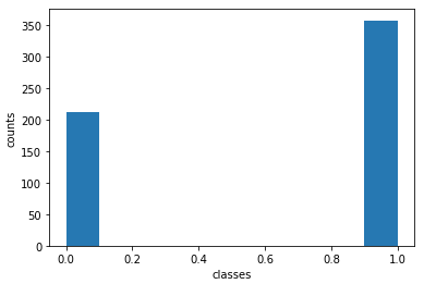
Percentage of y=0: 0.37258347978910367
Percentage of y=1: 0.6274165202108963
It’s evident that the dataset is somewhat unbalanced, with approx. 63% of the samples belonging to the benign class (y=1), and the remaining 37% belonging to the malignant class (y=0). We want to have our tree trained on a balanced dataset, as such when I choose training samples I will deliberately ensure I have an equal amount of samples from both classes. I want to use 60% of the data for training, and 40% for testing.
# partition the training data by label
y0 = y[y==0]
y1 = y[y==1]
X0 = X[y==0]
X1 = X[y==1]
# select the elements to remove at random
idx0 = np.random.choice([i for i in range(y0.shape[0])],size=nsampclass,replace=False)
idx1 = np.random.choice([i for i in range(y1.shape[0])],size=nsampclass,replace=False)
# select samples for training
y_train0 = y0[idx0]
y_train1 = y1[idx1]
X_train0 = X0[idx0,:]
X_train1 = X1[idx1,:]
y_train  = np.concatenate((y_train0,y_train1))
X_train  = np.concatenate((X_train0,X_train1))
# use remainder for testing
y_test0 = np.delete(y0,idx0)
y_test1 = np.delete(y1,idx1)
X_test0 = np.delete(X0,idx0,axis=0)
X_test1 = np.delete(X1,idx1,axis=0)
y_test  = np.concatenate((y_test0,y_test1))
X_test  = np.concatenate((X_test0,X_test1))
Now let’s check to verify that our training set is balanced:
# is the training dataset balanced now?
plt.hist(y_train)
plt.xlabel('classes')
plt.ylabel('counts')
plt.show()
print('Percentage of y=0: ',y_train[y_train==0].shape[0]/y_train.shape[0])
print('Percentage of y=1: ',y_train[y_train==1].shape[0]/y_train.shape[0])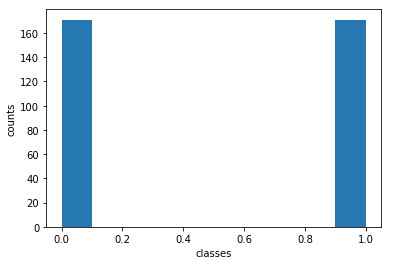
Percentage of y=0: 0.5
Percentage of y=1: 0.5
Great! We have a balanced training set. How does our test set look like:
# what is the proportion of class 0/1 in the test set?
plt.hist(y_test)
plt.xlabel('classes')
plt.ylabel('counts')
plt.show()
print('Percentage of y=0: ',y_test[y_test==0].shape[0]/y_test.shape[0])
print('Percentage of y=1: ',y_test[y_test==1].shape[0]/y_test.shape[0])

Percentage of y=0: 0.18061674008810572
Percentage of y=1: 0.8193832599118943
The test set is unbalanced, but this is understandable given the way the train/test split was done.
Test the Custom Decision Tree Classification Model
Now let’s declare a classifier, train it, and generate predictions:
# declare the classifier and train the model
clf = DecisionTreeClassifier(max_depth=5,loss='gini')
clf.train(X_train,y_train)
# generate predictions
yp = clf.predict(X_test)
Note that in this image we’ve defined a tree with a maximum of 5 levels, and makes use of the gini impurity metric.
To measure the performance of the classifier, we’ll make use of the accuracy, precision, and recall metrics. The best possible values for each of these metrics is 1, while the worst result is a 0. Let’s discuss these in a bit of detail.
Accuracy measures the fraction of correctly classified samples from the total sample set. This is expressed as:
Accuracy = \frac{TP + TN}{TP + FP + TN + FN} (12)
where TP, TN, FP, FN are the counts of True Positives, True Negatives, False Positives, and False Negatives, respectively.
Precision measures the ability of the model to correctly label positive values. Mathematically it is expressed by:
Precision = \frac{TP}{TP + FP} (13)
Recall measures the ability of the model to find all positive values. We can express as:
Recall = \frac{TP}{TP + FN} (14)
We can make use of the functions provided by scikit-learn to calculate (12), (13), and (14). Let’s now do that to compare the model predictions with the true class values:
# evaluate model performance
print("accuracy: %.2f" % accuracy_score(y_test,yp))
print("precision: %.2f" % precision_score(y_test,yp))
print("recall: %.2f" % recall_score(y_test,yp))
accuracy: 0.93
precision: 0.98
recall: 0.93
These look like good results for our classifier! The higher precision value likely results from the unbalanced nature of our test set.
Scikit-Learn Decision Tree Classification Model
To verify our model is functioning correctly, let’s compare its performance with the Decision Tree classifier provided by scikit-learn:
# import the scikit-learn model
from sklearn.tree import DecisionTreeClassifier
# declare the classifier and train the model
clf = DecisionTreeClassifier(max_depth=5,criterion='gini')
clf.fit(X_train,y_train)
DecisionTreeClassifier(max_depth=5)
# generate predictions
yp = clf.predict(X_test)
We can now evaluate this model the same way we did with our custom-built classifier:
# evaluate model performance
print("accuracy: %.2f" % accuracy_score(y_test,yp))
print("precision: %.2f" % precision_score(y_test,yp))
print("recall: %.2f" % recall_score(y_test,yp))
accuracy: 0.93
precision: 0.98
recall: 0.93
These results match those obtained with our custom classifier! We can run a few of these experiments by altering the hyper parameters selected for each of the models. Below is a table outlining the results obtained from the custom and scikit-learn classifiers7, with different choices for the impurity metric and maximum tree depth:
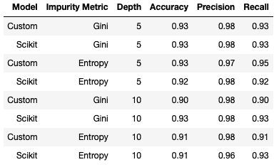
Note I left min_samples_split to its default value during these trials. Based on these results, we can see that these models having approximately the same level of performance. There is a slight degradation with maximum tree depth set to 10, indicating that our model has overfit the training set.
The Regression Dataset
Let’s now move on to test the regression Decision Tree. For data, we can use the make_regression functionality from scikit-learn to generate a toy dataset to work with:
# create a regression dataset
X,y = make_regression(n_samples=1000, n_features=8, n_informative=5, n_targets=1, noise=1, random_state=42)
# do train/test split
X_train, X_test, y_train, y_test = train_test_split(X, y, test_size=0.3, random_state=42)
Here we’ve created a dataset with 1000 samples comprised of 8 input features. Only 5 of these features are informative, however. We have 1 target label, and we also introduce a bit of noise into these data (with a standard deviation of 1). Finally a train/test split is done, with 30% of these data being reserved for the test set.
To evaluate the model performance, I’ll be using the root-mean-squared-error, mean-absolute-error, and r2 metrics. Let’s take a closer look at each of these:
Root Mean Squared Error (RMSE) is the root of the mean squared error. In turn, the mean squared error is the average of the square of the errors, and this quantity tends to be more sensitive to outliers in the results. Taking the root of the mean squared error ensures the units are the same as the dependant variable. Mathematically, this is expressed as:
RMSE = \sqrt{\frac{1}{N}\sum_i^N(y_{i,pred}-y_{i,true})^2} (15)
where y_{pred} are the predicted values, y_{true} are the true values, and N is the total number of samples considered in the calculation. The lowest possible value is 0, indicating no deviation between the predicted and true values.
Mean Absolute Error (MAE) is the average of the absolute value of the errors. This metric is also in the same units as the dependent variable, and is more easily interpretable as the average deviation of the model from the true values. This can be expressed as:
MAE = \frac{1}{N}\sum_i^N|y_{i,pred}-y_{i,true}| (16)
The lowest possible value is again 0, indicating no deviation between the predicted and true values.
R2 / Coefficient of Determination compares the variance in the data unexplained by the model, to the total variance in the data. This can be quantified as:
R^2 = 1 – \frac{\textrm{Unexplained} \quad \textrm{Variation}}{\textrm{Total} \quad \textrm{Variation}} (17)
The value of this metric can range from 0 to 1, indicating the worst and best possible outcomes, respectively.
Scikit-learn also provides functions to calculate (15), (16), and (17), which we will use here.
Test the Custom Decision Tree Regression Model
Let’s now declare our custom regressor, train the model, and generate predictions:
# declare the regressor and train the model
rgr = DecisionTreeRegressor(max_depth=5,loss='mae')
rgr.train(X_train,y_train)
# make predictions
yp = rgr.predict(X_test)
# evaluate model performance
print("rmse: %.2f" % np.sqrt(mean_squared_error(y_test,yp)))
print("mae: %.2f" % mean_absolute_error(y_test,yp))
print("r2: %.2f" % r2_score(y_test,yp))
rmse: 70.04
mae: 56.44
r2: 0.68
The model shown here has the settings of max_depth = 5 and the choice of the MAE impurity metric.
Scikit-Learn Decision Tree Regression Model
In the same way as we did with the classifier, we can compare these results with those obtained using the Decision Tree regressor available through scikit-learn:
# import the scikit-learn model
from sklearn.tree import DecisionTreeRegressor
# declare the regressor and train the model
rgr = DecisionTreeRegressor(max_depth=5,criterion='mae')
rgr.fit(X_train,y_train)
DecisionTreeRegressor(criterion=’mae’, max_depth=5)
# make predictions
yp = rgr.predict(X_test)
# evaluate model performance
print("rmse: %.2f" % np.sqrt(mean_squared_error(y_test,yp)))
print("mae: %.2f" % mean_absolute_error(y_test,yp))
print("r2: %.2f" % r2_score(y_test,yp))
rmse: 63.68
mae: 49.35
r2: 0.74
For this particular example, we can see that the scikit-learn model performs better than our custom-built regressor. We can run our comparison for various choices of hyper parameters, below I have compiled a table with various choices for maximum tree depth and impurity metric:
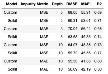
You may have noticed that there is a MAE for the impurity metric and for the model evaluation, equations (11) and (16), respectively. Both quantities have a similar form, but there is a difference:
- The impurity metric is computed with respect to the mean of the target values for any given node in the tree.
- The evaluation metric is computed by taking the difference between the predicted and actual target values for the entire test set.
For 75% of the configurations tested, the scikit-learn regressor outperforms our custom built-model. A noteworthy exception is the {impurity=MAE, depth=10} setup, which was also the best performing model overall. It is possible the replacing equation (9) with the median for each node in the tree could improve the results for our custom-built model. Feel free to try it out!
Final Remarks and Video
In this article you’ve learned:
- The motivation behind the Decision Tree model and when it was developed.
- The mathematical basis behind Decision Trees.
- How to build a Decision Tree in Python, along with some fundamentals behind object-oriented programming.
- How to use the Decision Tree functionality provided by the popular scikit-learn library.
I hope you enjoyed this article and gained some value from it! If you would like to take a closer look at the code presented here please take a look at my GitHub.
You can also watch me work through the content in this post here:
Related Posts
Addendum
Non-parametric models consist of algorithms that become more complex as the number of samples in the available data increases. By contrast, linear and logistic regression models are examples of parametric models, since their architecture is predefined and does not change with the size of the available dataset.
Kass, Gordon V. 1980. An Exploratory Technique for Investigating Large Quantities of Categorical Data, Applied Statistics, Vol. 29, No. 2: 119-127
Leo Breiman, Jerome Friedman, Richard A. Olshen, Charles J. Stone 1984. Classification and Regression Trees, CRC, ISBN 10: 0-412-04841-8
Quinlan, J.R. 1986. Induction of Decision Trees. Machine Learning 1: 81-106, 1986
Quinlan, J.R. 1993. Programs for Machine Learning. Machine Learning 16: 235-240, 1994
Balancing can be achieved either by ensuring an equal number of samples are obtained from each class, or by employing bagging/boosting techniques to address this problem. Alternatively, samples from under-represented classes can be weighted to counter the imbalance.
You can expect to have slightly different results if you rerun the code on your own machine when compared to those indicated in the table: the random nature of the train/test split largely accounts for this.
Hi I'm Michael Attard, a Data Scientist with a background in Astrophysics. I enjoy helping others on their journey to learn more about machine learning, and how it can be applied in industry.
[…] feature of Decision Trees results from how these models are built. In a previous article I covered the CART Decision Tree algorithm, and how it can be implemented in Python from scratch. […]
[…] we will focus strictly on CART. I covered the details of the CART Decision Tree algorithm in a previous article. With this approach, the input dataset is split into a series of subsets according to decision […]
[…] an earlier article, I covered in depth the CART algorithm, and how to implement this in Python. For that discussion, […]
[…] an earlier article, I covered in depth the CART algorithm, and how to implement this in Python. For that discussion, […]
[…] a previous article, I covered in detail the CART Decision Tree algorithm. One of the main considerations listed in […]
[…] Decision Trees are generally quite intuitive to understand, and easy to interpret. Unlike most other machine […]
[…] Decision Trees are supervised machine learning algorithms that are fairly easy to visualise and interpret. Their interpretability is not affected by the dimensionality of the data either. As such, we can make use of a Decision Tree classifier to assist in explaining the clustering results. […]
[…] aim of this pipeline will be to make use of a Decision Tree Regressor to predict housing values. We will make use of the California Housing Prices dataset. These data […]
[…] simple example would be to consider how Decision Trees are built. Deciding how splits are done, at a specific node, is learned during training and so […]