Build a Random Forest in Python from Scratch

For this post, we will Build a Random Forest in Python from scratch. I will include examples in classification and regression.

Motivation to Build a Random Forest Model

Bagging ensembles are an approach to reduce variance, and thereby increase model performance. In this algorithm, multiple weak learner models produce predictions on a series of bootstrap samples. Normally, the weak learners are decision trees. Combining the different predictions achieves variance reduction.

There is a potential pitfall for the bagging algorithm: the possibility of a small subset of features, in the input data, dominating over all others. In this case, each weak learner will place most of the weight on this subset of features during training. As a result, the weak learners will become correlated. This will diminish the potential performance benefits of using an ensemble.

Random Forest is another ensemble algorithm that is closely related to bagging ensembles. Both utilise bootstrapped samples, and both combine the output of multiple weak learners. The Random Forest algorithm distinguishes itself by introducing an additional layer of random data selection for each constituent decision tree. For each node in these trees, splitting is done using a random subset of all the features. This ensures that the resulting trees in the ensemble are uncorrelated.

The Random Forest algorithm was developed in 2001 by Leo Breiman. It has become a popular machine learning model for business applications due to the quality of predictions they can generate, while requiring relatively little in terms of preparation to setup. The downside is that it is much harder to explain how this algorithm works to a non-technical audience, as opposed to a single decision tree.

Assumptions and Considerations for Random Forests

Random Forests are closely related to bagging ensembles, where both rely on bootstrapped samples from the input training data. As such, the assumptions discussed in the bagging and bootstrap method articles still hold here.

There is a subtile distinction between bagging ensembles and random forests. Bagging ensembles could technically use any model for its weak learners. On the other hand, random forests always use (modified) decision trees. As such, we make no assumptions on the distributions in the data. Furthermore, minimal data preparation is necessary. At the same time, the key weakness of decision trees, namely their tendency to be instable to small variations in the dataset, are an asset to the ensemble: allowing it to explore the solution space of the problem.

Despite the advantages, there are some key points to keep in mind when using random forests:

We may need to account for missing or NaN values, depending on the implementation
Since a random forest is an ensemble of many decision trees, training a random forest can take substantially more time then a singular model
For classification problems, decision trees can have bias in cases of unbalanced data. Therefore, the dataset should be balanced prior to training a random forest classifier

Derivation of the Random Forest Algorithm

Let’s begin by assuming we have some data with which to work. These data will be composed of independent $\bold{X}$ and dependent $\bold{y}$ variables:

$\bold{y} = \begin{bmatrix} y_1 \\ y_2 \\ . \\ . \\ . \\ y_N \end{bmatrix}$ , $\bold{X} = \begin{bmatrix} x_{1,1} & x_{1,2} & … & x_{1,M} \\ x_{2,1} & x_{2,2} & … & x_{2,M} \\ … & … & … & … \\ … & … & … & … \\ x_{N,1} & x_{N,2} & … & x_{N,M} \end{bmatrix}$ (1)

There are $M$ features in this dataset, along with a total of $N$ samples. Our aim will be to build a model that can accurately predict values in $\bold{y}$ from samples in $\bold{X}$ . The feature set is defined by the column vectors $\{ \bold{x}_f \}$ that make up $\bold{X}$ , where $f = 1..M$ . We can combine $\bold{X}$ and $\bold{y}$ into a total data matrix:

$\bold{D} = \begin{bmatrix} x_{1,1} & x_{1,2} & … & x_{1,M} & y_1 \\ x_{2,1} & x_{2,2} & … & x_{2,M} & y_2 \\ … & … & … & … & … \\ … & … & … & … & … \\ x_{N,1} & x_{N,2} & … & x_{N,M} & y_N \end{bmatrix}$ (2)

To solve the modelling problem, we will build a set of uncorrelated decision trees. Each tree will make predictions on unseen data. Next the algorithm combines these predictions, to yield a result for the entire ensemble. The key challenge here is to generate uncorrelated decision trees: since CART follows a greedy algorithm, it is possible that our trees could all have a similar structure if a small subset of our $M$ features dominate in terms of the optimisation procedure. I illustrate here what we want:

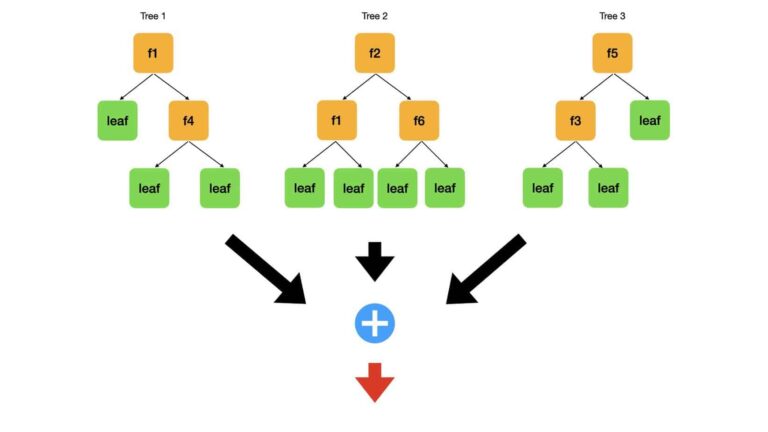
Depicted here is a small random forest that consists of just 3 trees. A dataset with 6 features (f1…f6) is used to fit the model. Each tree is drawn with interior nodes¹ (orange), where the data is split, and leaf nodes (green) where a prediction is made. Notice the split feature is written on each interior node (i.e. ‘f1‘). Each of the 3 trees has a different structure. This is true in terms of the distribution of the nodes, and features used while splitting. The algorithm generates predictions from these trees (black arrows) and combines them (blue addition circle). Next the algorithm makes a final set of results (red arrow).

So how do we build a Random Forest?

The algorithm for classification, or regression, random forests is as follows:

Perform a train – test split of the available data $\bold{D}$
Set the desired size of the ensemble (i.e. the number of trees to include in the random forest) $B$ , and select an impurity metric that will be used to build each decision tree (I described a few impurity metrics in an earlier article on decision trees)
Produce $B$ bootstrap samples on the training data
Loop through each of the b = 1..B bootstrap samples:
- - Build a modified decision tree T_b on the bootstrap sample b by recursively repeating the following steps. This process is stopped when the data can no longer be split, either because all samples in the current node have the same label, or because some regularisation threshold has been reached:
    - randomly choose a subset of $M_{sub}$ features from the total set of $M$ features in the input data. Typically $M_{sub}=\sqrt{M}$
    - choose one feature $f^*$ from the selected set of $M_{sub}$ features, and a corresponding threshold value $x_{f^*}$ for $f^*$ , by which the training data will be split. The choice $\{f^*,x_{f^*}\}$ is made that minimises the chosen impurity metric
    - split the data available at the current node $\bold{D}_{node}$ based upon the values of $\{f^*,x_{f^*}\}$ : $\bold{D}_{left} = \bold{D}_{node}|\bold{x}_{f^*} \leq x_{f^*}$ and $\bold{D}_{right} = \bold{D}_{node}|\bold{x}_{f^*} > x_{f^*}$ . Pass $\bold{D}_{left}$ and $\bold{D}_{right}$ to the child nodes
  - Store the trained decision tree $T_b$ .
  - (Optional) Store the out-of-bag (oob) samples for the current bootstrap iteration $b$ . Generate predictions for the oob samples using $T_b$ , and compare them to the label values. Store the results of the comparison.
Return the trained ensemble of $T_{1..B}$ trees. If the analysis on the oob samples was performed, the results can now be used to compute standard errors for the ensemble
To generate predictions on unseen/test data, pass the data to each of the $T_{1..B}$ trees and generate $B$ sets of predictions. Combine the $B$ sets of predictions, either through majority voting (classification) or by computing the mean/median (regression)

The key distinction between CART, and the modified decision trees $T_b$ discussed here, is the step set in bold. The end result is a set of $T_{1..B}$ trees with various different architectures that are not correlated, and can therefore cover the solution space of the problem. Combining their results can lower the variance in the results, as opposed to using a singular decision tree.

Build and Test Random Forest in Python

In the following sub-sections, we will build random forest models from scratch using Python 3. These implementations will then be tested on publicly available data. The test results will be used to compare the performance of our implementation to the scikit-learn random forest, bagging ensemble, and decision tree models.

Disclaimer: re-running the following code could produce slightly different results, due to the random nature of the processes involved.

Import Required Packages

Here we’ll build both classification and regression random forests in Python. The datasets we will use are available through scikit-learn. For classification, we will use the wine quality dataset. For regression, the boston housing prices dataset will be used.

We can begin with importing the necessary packages:

## imports ##
import numpy as np
import pandas as pd
import seaborn as sn
import matplotlib.pyplot as plt
from sklearn.base import clone
from sklearn.datasets import load_wine,load_boston
from sklearn.model_selection import StratifiedKFold,cross_validate
from sklearn.metrics import accuracy_score,precision_score,recall_score,mean_absolute_error,mean_squared_error,r2_score,make_scorer
from abc import ABC,abstractmethod
from decisiontrees import DecisionTreeClassifier, DecisionTreeRegressor

The last package I import from, decisiontrees, is a custom Python package I have created to implement the modified decision trees $T_b$ described in the previous section. The classification and regression trees implemented here are based upon the code described in an earlier article on decision trees. You can view the complete implementation of the decisiontrees package on the inside learning machines git repository.

There are two key additions that I introduce in the decisiontrees package, versus the code I implemented earlier in the decision tree article:

Only a subset of $M_{sub}$ features, from the total $M$ , are made available to the algorithm at any given node in the tree. The algorithm is only permitted to split the data with one of the $M_{sub}$ features. This change is implemented in the __grow function, line 82 in base_tree.py. Note that $M_{sub} = \sqrt{M}$ .
DecisionTreeClassifier has one additional input boolean argument, balance_class_weights. When this is set to True, class weights are assigned that are inversely proportional to the frequency of the class in the labels $\bold{y}$ . If False, all classes receive weight of 1. These weights are calculated inside the fit function, line 74 in treeclassifier.py

Build Random Forest Base Class

Now we will create a base class for the random forest implementation:

#base class for the random forest algorithm
class RandomForest(ABC):
    #initializer
    def __init__(self,n_trees=100):
        self.n_trees = n_trees
        self.trees   = []

Our base class is RandomForest, with the object ABC passed as a parameter. The function __init__(self,n_trees=100) initialises the class instance, and takes the argument n_trees that sets the size of the ensemble to create.

    #private function to make bootstrap samples
    def __make_bootstraps(self,data):
        #initialize output dictionary & unique value count
        dc   = {}
        unip = 0
        #get sample size
        b_size = data.shape[0]
        #get list of row indexes
        idx = [i for i in range(b_size)]
        #loop through the required number of bootstraps
        for b in range(self.n_trees):
            #obtain boostrap samples with replacement
            sidx   = np.random.choice(idx,replace=True,size=b_size)
            b_samp = data[sidx,:]
            #compute number of unique values contained in the bootstrap sample
            unip  += len(set(sidx))
            #obtain out-of-bag samples for the current b
            oidx   = list(set(idx) - set(sidx))
            o_samp = np.array([])
            if oidx:
                o_samp = data[oidx,:]
            #store results
            dc['boot_'+str(b)] = {'boot':b_samp,'test':o_samp}
        #return the bootstrap results
        return(dc)

The private² function __make_bootstraps(self, data) is used to generate the desired number of bootstrap samples, which is the same as the number of trees in the ensemble. It takes one argument, data, which is a numpy 2D array containing the provided training data. This function is essentially the same to the one discussed in the bootstrap algorithm article.

    #public function to return model parameters
    def get_params(self, deep = False):
        return {'n_trees':self.n_trees}

    #protected function to obtain the right decision tree
    @abstractmethod
    def _make_tree_model(self):
        pass

get_params(self,deep=False) : this function is used to return the parameters of the class instance
_make_tree_model(self) : this protected function is an abstract method, and will be implemented in the child classes

    #protected function to train the ensemble
    def _train(self,X_train,y_train):
        #package the input data
        training_data = np.concatenate((X_train,y_train.reshape(-1,1)),axis=1)
        #make bootstrap samples
        dcBoot = self.__make_bootstraps(training_data)
        #iterate through each bootstrap sample & fit a model ##
        tree_m = self._make_tree_model()
        dcOob    = {}
        for b in dcBoot:
            #make a clone of the model
            model = clone(tree_m)
            #fit a decision tree model to the current sample
            model.fit(dcBoot[b]['boot'][:,:-1],dcBoot[b]['boot'][:,-1].reshape(-1, 1))
            #append the fitted model
            self.trees.append(model)
            #store the out-of-bag test set for the current bootstrap
            if dcBoot[b]['test'].size:
                dcOob[b] = dcBoot[b]['test']
            else:
                dcOob[b] = np.array([])
        #return the oob data set
        return(dcOob)

The protected function _train(self,X_train,y_train) is used to generate the bootstrap samples required, and grow all the trees in the ensemble. The arguments X_train and y_train are the independent and dependent variables, respectively.

    #protected function to predict from the ensemble
    def _predict(self,X):
        #check we've fit the ensemble
        if not self.trees:
            print('You must train the ensemble before making predictions!')
            return(None)
        #loop through each fitted model
        predictions = []
        for m in self.trees:
            #make predictions on the input X
            yp = m.predict(X)
            #append predictions to storage list
            predictions.append(yp.reshape(-1,1))
        #compute the ensemble prediction
        ypred = np.mean(np.concatenate(predictions,axis=1),axis=1)
        #return the prediction
        return(ypred)

The final function in this class is _predict(self,X), a protected member function used to generate predictions for the ensemble. The predictions from the various trees are combined by calculating the mean. The argument X is the set of independent variables upon which the predictions will be based.

Build Random Forest Classifier

Now the child classes will be implemented. First we will start with the random forest classifier:

#class for random forest classifier
class RandomForestClassifier(RandomForest):
    #initializer
    def __init__(self,n_trees=100,max_depth=None,min_samples_split=2,loss='gini',balance_class_weights=False):
        super().__init__(n_trees)
        self.max_depth             = max_depth
        self.min_samples_split     = min_samples_split
        self.loss                  = loss
        self.balance_class_weights = balance_class_weights

The class RandomForestClassifier is defined as a child class, with the object RandomForest passed as a parameter. The function:

__init__(self,n_trees=100,max_depth=None,min_samples_split=2,loss=‘gini’,balance_class_weights=False)

initialises the class instance, and takes the arguments n_trees, max_depth, min_samples_split, loss, and balance_class_weights. Like in the base class, n_trees sets the size of the ensemble. The argument max_depth sets the maximum depth to grow the trees, while min_samples_split defines the minimum number of samples required for a node split. The loss, or impurity function, used while growing the trees is set by loss. Finally, balance_class_weights is a boolean used to activate the internal functionality to account for unbalanced classes in the data.

    #protected function to obtain the right decision tree
    def _make_tree_model(self):
        return(DecisionTreeClassifier(max_depth             = self.max_depth,
                                      min_samples_split     = self.min_samples_split,
                                      loss                  = self.loss,
                                      balance_class_weights = self.balance_class_weights))
    
    #public function to return model parameters
    def get_params(self, deep = False):
        return {'n_trees':self.n_trees,
                'max_depth':self.max_depth,
                'min_samples_split':self.min_samples_split,
                'loss':self.loss,
                'balance_class_weights':self.balance_class_weights}

_make_tree_model(self) : protected function that builds a decision tree classifier with the input arguments obtained from the initialiser
get_params(self,deep=False) : function used to return the parameters of the class instance

    #train the ensemble
    def fit(self,X_train,y_train,print_metrics=False):
        #call the protected training method
        dcOob = self._train(X_train,y_train)
        #if selected, compute the standard errors and print them
        if print_metrics:
            #initialise metric arrays
            accs = np.array([])
            pres = np.array([])
            recs = np.array([])
            #loop through each bootstrap sample
            for b,m in zip(dcOob,self.trees):
                #compute the predictions on the out-of-bag test set & compute metrics
                if dcOob[b].size:
                    yp  = m.predict(dcOob[b][:,:-1])
                    acc = accuracy_score(dcOob[b][:,-1],yp)
                    pre = precision_score(dcOob[b][:,-1],yp,average='weighted')   
                    rec = recall_score(dcOob[b][:,-1],yp,average='weighted')
                    #store the error metrics
                    accs = np.concatenate((accs,acc.flatten()))
                    pres = np.concatenate((pres,pre.flatten()))
                    recs = np.concatenate((recs,rec.flatten()))
            #print standard errors
            print("Standard error in accuracy: %.2f" % np.std(accs))
            print("Standard error in precision: %.2f" % np.std(pres))
            print("Standard error in recall: %.2f" % np.std(recs))

The function:

fit(self,X_train,y_train,print_metrics=False)

is used to train the ensemble classifier. The arguments X_train and y_train are arrays that contain the independent and dependent variables, respectively. The boolean print_metrics controls whether the standard error statistics are printed out after training is completed.

    #predict from the ensemble
    def predict(self,X):
        #call the protected prediction method
        ypred = self._predict(X)
        #convert the results into integer values & return
        return(np.round(ypred).astype(int))

The last member function of the random forest classifier is:

predict(self,X)

As its namesake suggests, this function is used to generate predictions from the ensemble. Note that this function calls the protected _predict method function inherited from the base class, and then subsequently converts the predictions into integers.

Build Random Forest Regressor

The last class we will define here is the one for the random forest regressor. Since the functionality of this class is very similar to that of the classifier (only adapted for regression), I will post the code for this class here in a single block:

#class for random forest regressor
class RandomForestRegressor(RandomForest):
    #initializer
    def __init__(self,n_trees=100,max_depth=None,min_samples_split=2,loss='mse'):
        super().__init__(n_trees)
        self.max_depth             = max_depth
        self.min_samples_split     = min_samples_split
        self.loss                  = loss
        
    #protected function to obtain the right decision tree
    def _make_tree_model(self):
        return(DecisionTreeRegressor(self.max_depth,self.min_samples_split,self.loss))
    
    #public function to return model parameters
    def get_params(self, deep = False):
        return {'n_trees':self.n_trees,
                'max_depth':self.max_depth,
                'min_samples_split':self.min_samples_split,
                'loss':self.loss}
    
    #train the ensemble
    def fit(self,X_train,y_train,print_metrics=False):
        #call the protected training method
        dcOob = self._train(X_train,y_train)
        #if selected, compute the standard errors and print them
        if print_metrics:
            #initialise metric arrays
            maes = np.array([])
            mses = np.array([])
            r2ss = np.array([])
            #loop through each bootstrap sample
            for b,m in zip(dcOob,self.trees):
                #compute the predictions on the out-of-bag test set & compute metrics
                if dcOob[b].size:
                    yp  = m.predict(dcOob[b][:,:-1])
                    mae = mean_absolute_error(dcOob[b][:,-1],yp)
                    mse = mean_squared_error(dcOob[b][:,-1],yp)   
                    r2s = r2_score(dcOob[b][:,-1],yp)
                    #store the error metrics
                    maes = np.concatenate((maes,mae.flatten()))
                    mses = np.concatenate((mses,mse.flatten()))
                    r2ss = np.concatenate((r2ss,r2s.flatten()))
            #print standard errors
            print("Standard error in mean absolute error: %.2f" % np.std(maes))
            print("Standard error in mean squred error: %.2f" % np.std(mses))
            print("Standard error in r2 score: %.2f" % np.std(r2ss))
            
    #predict from the ensemble
    def predict(self,X):
        #call the protected prediction method
        ypred = self._predict(X)
        #return the results
        return(ypred)

Some notable points:

The protected function _make_tree_model(self) returns a decision tree regressor
fit(self,X_train,y_train,print_metrics=False) prints regression metrics when print_metrics=True
predict(self,X) returns the mean predictions from the inherited protected function _predict

Random Forest Classifier - Wine Quality Dataset

Data Exploration

To test out the classifier we’ve built, let’s use the wine quality dataset available through scikit-learn:

#load the wine dataset
dfX,sY = load_wine(return_X_y=True, as_frame=True)

#check the dimensions of these data
print('Dimensions of X: ',dfX.shape)
print('Dimensions of y: ',sY.shape)

Dimensions of X: (178, 13)

Dimensions of y: (178,)

#what unique classes exist in the label variable?
print('Classes in the label: ',sY.unique())

Classes in the label: [0 1 2]

These data consist of 178 samples, with 13 independent features. The dependent variable consists of 3 different labels, corresponding to the quality of the wine. Let’s plot the distribution of these classes:

#what is the frequency of the classes in the dataset?
sY.hist()
plt.show()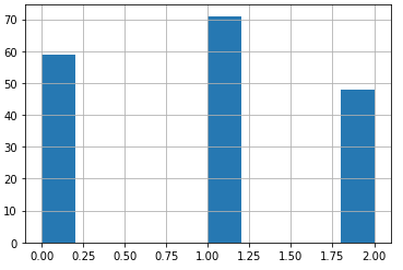

The classes are not balanced, although the frequency differences are not severe. Let’s now move ahead and investigate the distributions and correlations in the independent features:

#make a boxplot to view the distribution in these data
dfX.boxplot(figsize=(20,10),rot=45)
plt.show()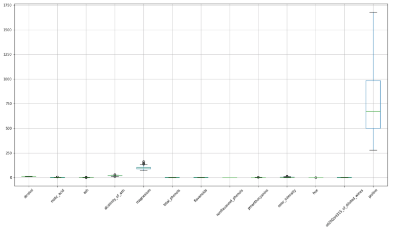

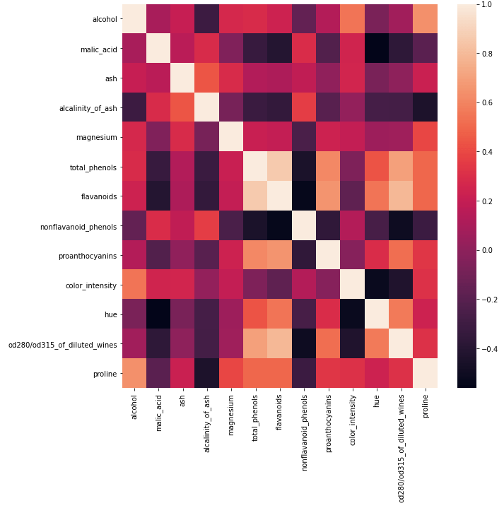
## plot the pearson correlation for our input features ##
fig, ax = plt.subplots(figsize = (10, 10)) 
dfCorr  = dfX.corr() 
sn.heatmap(dfCorr) 
plt.show()

The spreads in these data vary from feature to feature, and we can see that different units also apply to each feature. However, the box plots indicate that there are almost no outliers.

The heat map appears to indicate some of our independent features are highly correlated. Let’s take a closer look to see how many of them are present:

#convert all correlations to positive values
dfCorr = dfCorr.abs()

#loop through rows
for index, sRow in dfCorr.iterrows():
    #get the valid entries
    sCorrs = sRow[sRow.index != index]
    sCorrs = sCorrs[sCorrs > 0.8]
    #print out results
    if not sCorrs.empty:
        print('highly correlated input features: ',index,' & ',sCorrs.index.values)

highly correlated input features: total_phenols & [‘flavanoids’]

highly correlated input features: flavanoids & [‘total_phenols’]

Here I’m listing all feature pairs that exceed an absolute correlation coefficient of 0.8. Only two features exceed this threshold: total_phenols & flavanoids. In situations where a large number of features are present (1000’s or more), we could remove 1 feature per pair to reduce the dimensionality of the data. However, with this dataset we can safely proceed without dropping any features.

Modelling with a Random Forest Classifier

Now we can attempt to model these data with the random forest classifier we have built. Let’s create an instance with balance_class_weights set to True, and train it to view the standard error estimates for our predictions:

#create a random forest with balance class weights enabled
rfc = RandomForestClassifier(balance_class_weights=True)

## train the ensemble & view estimates for prediction error ##
rfc.fit(dfX.values,sY.values,print_metrics=True)

Standard error in accuracy: 0.06

Standard error in precision: 0.05

Standard error in recall: 0.06

The standard errors look reasonable. To properly assess the performance of the model, I will use a 10-fold cross validation:

## use k fold cross validation to measure performance ##
scoring_metrics = {'accuracy': make_scorer(accuracy_score), 
                   'precision': make_scorer(precision_score, average='weighted'),
                   'recall': make_scorer(recall_score, average='weighted')}
dcScores        = cross_validate(rfc,dfX.values,sY.values,cv=StratifiedKFold(10),scoring=scoring_metrics)
print('Mean Accuracy: %.2f' % np.mean(dcScores['test_accuracy']))
print('Mean Precision: %.2f' % np.mean(dcScores['test_precision']))
print('Mean Recall: %.2f' % np.mean(dcScores['test_recall']))

Mean Accuracy: 0.97

Mean Precision: 0.97

Mean Recall: 0.97

These results look quite good! It’s important to note that besides balance_class_weights, all other arguments to the model were kept at their default values.

Comparing the Built Random Forest Classifier with Scikit-Learn Models

We can now compare the performance of our classifier to models available through scikit-learn. Let’s import the Random Forest Classifier, Bagging Classifier, and Decision Tree Classifier:

## import the scikit-learn models ##
from sklearn.ensemble import RandomForestClassifier, BaggingClassifier 
from sklearn.tree import DecisionTreeClassifier

The comparison will start with the scikit-learn random forest classifier:

#create a random forest with balanced class weights
rfc = RandomForestClassifier(class_weight='balanced')

## use k fold cross validation to measure performance ##
scoring_metrics = {'accuracy': make_scorer(accuracy_score), 
                   'precision': make_scorer(precision_score, average='weighted'),
                   'recall': make_scorer(recall_score, average='weighted')}
dcScores        = cross_validate(rfc,dfX.values,sY.values,cv=StratifiedKFold(10),scoring=scoring_metrics)
print('Mean Accuracy: %.2f' % np.mean(dcScores['test_accuracy']))
print('Mean Precision: %.2f' % np.mean(dcScores['test_precision']))
print('Mean Recall: %.2f' % np.mean(dcScores['test_recall']))

Mean Accuracy: 0.98

Mean Precision: 0.98

Mean Recall: 0.98

Like with our custom random forest classifier, here I’ve done a 10-fold cross validation analysis. As we may expect, the results obtained here with the scikit-learn model are very similar to those we obtained previously. This confirms our custom built model has been implemented correctly.

Now let’s repeat this analysis, using the bagging classifier and decision tree classifier:

#create a bagging classifer with balanced class weights
btc = BaggingClassifier(base_estimator=DecisionTreeClassifier(class_weight='balanced'),n_estimators=100)

## use k fold cross validation to measure performance ##
scoring_metrics = {'accuracy': make_scorer(accuracy_score), 
                   'precision': make_scorer(precision_score, average='weighted'),
                   'recall': make_scorer(recall_score, average='weighted')}
dcScores        = cross_validate(btc,dfX.values,sY.values,cv=StratifiedKFold(10),scoring=scoring_metrics)
print('Mean Accuracy: %.2f' % np.mean(dcScores['test_accuracy']))
print('Mean Precision: %.2f' % np.mean(dcScores['test_precision']))
print('Mean Recall: %.2f' % np.mean(dcScores['test_recall']))

Mean Accuracy: 0.94

Mean Precision: 0.95

Mean Recall: 0.94

#create a decision tree classifer with balanced class weights
dtc = DecisionTreeClassifier(class_weight='balanced')

## use k fold cross validation to measure performance ##
scoring_metrics = {'accuracy': make_scorer(accuracy_score), 
                   'precision': make_scorer(precision_score, average='weighted'),
                   'recall': make_scorer(recall_score, average='weighted')}
dcScores        = cross_validate(dtc,dfX.values,sY.values,cv=StratifiedKFold(10),scoring=scoring_metrics)
print('Mean Accuracy: %.2f' % np.mean(dcScores['test_accuracy']))
print('Mean Precision: %.2f' % np.mean(dcScores['test_precision']))
print('Mean Recall: %.2f' % np.mean(dcScores['test_recall']))

Mean Accuracy: 0.89

Mean Precision: 0.92

Mean Recall: 0.89

The following table summarises the results:

Model	Accuracy	Precision	Recall
Custom Random Forest	0.97	0.97	0.97
Scikit-Learn Random Forest	0.98	0.98	0.98
Scikit-Learn Bagging Classifier	0.94	0.95	0.94
Scikit-Learn Decision Tree Classifier	0.89	0.92	0.89

As would be expected, the random forest classifiers perform better than the bagging classifier. Both the random forests and bagging classifier perform better than the decision tree classifier. These results show the progression in model improvement as steps are increasingly taken to account for variance in the algorithm. We start with a simple decision tree, move on to using an ensemble of trees with bootstrapped samples (bagging) and finally end with an ensemble of uncorrelated trees with bootstrapped samples (random forest).

Random Forest Regressor - Boston House Prices Dataset

Data Exploration

To test out the regressor we’ve built, let’s use the boston house prices dataset available through scikit-learn:

#load the boston dataset
data = load_boston()
#obtain input data
X = data.data
#obtain labels
Y = data.target
#obtain input labels
names = data.feature_names
#convert input features to dataframe
dfX = pd.DataFrame(X,columns=names)

Now that we have our data loaded into the notebook, let’s take an initial look at these data:

#check the dimensions of these data
print('Dimensions of X: ',dfX.shape)
print('Dimensions of y: ',Y.shape)

Dimensions of X: (506, 13)

Dimensions of y: (506,)

#produce a histogram of the target labels
plt.hist(Y)
plt.xlabel('Median Price $1000')
plt.ylabel('Frequency')
plt.title('Histogram of Boston House Prices in $1000')
plt.show()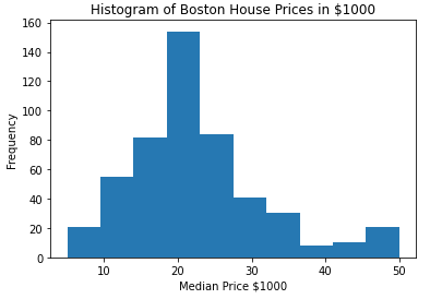

These data consist of 506 samples, with 13 independent features. The dependant variable is the median house price (in thousands of $USD), and its distribution peaks around $20K. However, a secondary minor peak also occurs around $50K. Note that these data were published in 1978, and as such reflect USD from that time period.

Let’s now investigate the distributions and correlations in the independent features for this dataset:

#make a boxplot to view the distribution in these data
dfX.boxplot(figsize=(20,10),rot=45)
plt.show()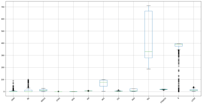

## plot the pearson correlation for our input features ##
fig, ax = plt.subplots(figsize = (10, 10)) 
dfCorr  = dfX.corr() 
sn.heatmap(dfCorr) 
plt.show()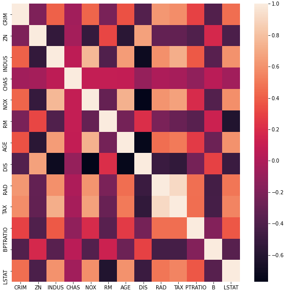

The spreads in these distributions vary from feature to feature, with many outliers present in CRIM, ZN, and B. Some of these features, most notably TAX, also show signs of a highly skewed distribution. In addition, the heat map indicates that some of these features are highly correlated.

Now we can work out which features show a high degree of collinearity (correlation coefficient greater than 0.8):

#convert all correlations to positive values
dfCorr = dfCorr.abs()

#loop through rows
for index, sRow in dfCorr.iterrows():
    #get the valid entries
    sCorrs = sRow[sRow.index != index]
    sCorrs = sCorrs[sCorrs > 0.8]
    #print out results
    if not sCorrs.empty:
        print('highly correlated input features: ',index,' & ',sCorrs.index.values)

highly correlated input features: RAD & [‘TAX’]

highly correlated input features: TAX & [‘RAD’]

Like the case we saw with the wine quality dataset, only two features are highly correlated: RAD and TAX. In a situation where our dataset consists of many features (1000’s or more), it would make sense to remove one of the highly correlated variables. However, this dataset only has 13 independent features, and as such we can proceed without having to worry about collinearity.

Modelling with a Random Forest Regressor

Now we can attempt to model these data with the random forest regressor we have built. Let’s create an instance, and train it to view the standard error estimates for our predictions:

#create a random forest with default values
rfr = RandomForestRegressor()

## train the ensemble & view estimates for prediction error ##
rfr.fit(dfX.values,Y,print_metrics=True)

Standard error in mean absolute error: 0.37

Standard error in mean squred error: 9.14

Standard error in r2 score: 0.11

The standard errors look reasonable. To properly assess the performance of the model, I will use a 10-fold cross-validation:

## use k fold cross validation to measure performance ##
scoring_metrics = {'mae': make_scorer(mean_absolute_error), 
                   'mse': make_scorer(mean_squared_error),
                   'r2': make_scorer(r2_score)}
dcScores        = cross_validate(rfr,dfX.values,Y,cv=10,scoring=scoring_metrics)
print('Mean MAE: %.2f' % np.mean(dcScores['test_mae']))
print('Mean MSE: %.2f' % np.mean(dcScores['test_mse']))
print('Mean R2: %.2f' % np.mean(dcScores['test_r2']))

Mean MAE: 3.05

Mean MSE: 21.47

Mean R2: 0.55

These result look sensible. Note that no hyperparameter tuning was done, like the case with the random forest classifier.

Comparing the Built Random Forest Regressor with Scikit-Learn Models

We can now compare the performance of our regressor to models available through scikit-learn. Let’s import the Random Forest Regressor, Bagging Regressor, and Decision Tree Regressor:

## import the scikit-learn models ##
from sklearn.ensemble import RandomForestRegressor, BaggingRegressor 
from sklearn.tree import DecisionTreeRegressor

The comparison will start with the scikit-learn random forest regressor:

#create a random forest with default values
rfr = RandomForestRegressor(max_features='sqrt')

## use k fold cross validation to measure performance ##
scoring_metrics = {'mae': make_scorer(mean_absolute_error), 
                   'mse': make_scorer(mean_squared_error),
                   'r2': make_scorer(r2_score)}
dcScores        = cross_validate(rfr,dfX.values,Y,cv=10,scoring=scoring_metrics)
print('Mean MAE: %.2f' % np.mean(dcScores['test_mae']))
print('Mean MSE: %.2f' % np.mean(dcScores['test_mse']))
print('Mean R2: %.2f' % np.mean(dcScores['test_r2']))

Mean MAE: 3.01

Mean MSE: 20.10

Mean R2: 0.55

Like with our custom random forest regressor, here I’ve done a 10-fold cross validation analysis. I’ve set max_features=‘sqrt’ to ensure the functionality here match the implementation in our custom model. As we may expect, the results obtained here with the scikit-learn model are very similar to those we obtained previously. This confirms our custom built model has been implemented correctly.

Now let’s repeat this analysis, using the bagging regressor and decision tree regressor:

#create a bagging regressor 
btr = BaggingRegressor(base_estimator=DecisionTreeRegressor(),n_estimators=100)

## use k fold cross validation to measure performance ##
scoring_metrics = {'mae': make_scorer(mean_absolute_error), 
                   'mse': make_scorer(mean_squared_error),
                   'r2': make_scorer(r2_score)}
dcScores        = cross_validate(btr,dfX.values,Y,cv=10,scoring=scoring_metrics)
print('Mean MAE: %.2f' % np.mean(dcScores['test_mae']))
print('Mean MSE: %.2f' % np.mean(dcScores['test_mse']))
print('Mean R2: %.2f' % np.mean(dcScores['test_r2']))

Mean MAE: 3.00

Mean MSE: 21.77

Mean R2: 0.51

#create a decision tree regressor 
dtr = DecisionTreeRegressor()

## use k fold cross validation to measure performance ##
scoring_metrics = {'mae': make_scorer(mean_absolute_error), 
                   'mse': make_scorer(mean_squared_error),
                   'r2': make_scorer(r2_score)}
dcScores        = cross_validate(dtr,dfX.values,Y,cv=10,scoring=scoring_metrics)
print('Mean MAE: %.2f' % np.mean(dcScores['test_mae']))
print('Mean MSE: %.2f' % np.mean(dcScores['test_mse']))
print('Mean R2: %.2f' % np.mean(dcScores['test_r2']))

Mean MAE: 3.98

Mean MSE: 38.95

Mean R2: -0.07

The following table summarises the results:

Model	MAE	MSE	R2
Custom Random Forest	3.05	21.47	0.55
Scikit-Learn Random Forest	3.01	20.10	0.55
Scikit-Learn Bagging Regressor	3.00	21.77	0.51
Scikit-Learn Decision Tree Regressor	3.98	38.95	-0.07

The results show that our custom built random forest regressor performs similarly to the model available through scikit-learn in terms of the MAE and coefficient of determination ( $R^2$ ) scores. The MSE result is a bit better with the scikit-learn model, indicating that this model is better at handling outliers. Here we see similar results to the classification example. There is a general trend of improved performance as more steps are taken to account for variance. The random forest algorithm performs better than the bagging regressor, in terms of MSE & $R^2$ . This implies that the random forest is somewhat less sensitive to outliers than the bagging regressor. In turn, both of these models perform better than the decision tree regressor.

Final Remarks

In this article you have learned:

The motivation behind the random forest algorithm
The logic behind random forests
How to build your own random forest classifiers and regressors in Python
How random forests compare to bagging ensembles and decision trees with the models available through the scikit-learn library

I hope you enjoyed this article and gained some value from it! If you would like to take a closer look at the code presented here please take a look at my git repository.

Addendum

Notice that for simplicity I include the root node as an interior node for each tree.
All the classes built in this article will follow the public, protected, and private convention for accessing resources:
- public member variables and functions of a class are accessible everywhere.
- protected member variables and functions of a class are accessible within the class, and to any child classes. You can see this by a single underscore, ‘_’ at the start of the member name.
- private member variables and functions of a class are only accessible within the class. You can see this by a double underscore, ‘__’ at the start of the member name.

5 1 vote

Article Rating

1 Comment

Oldest

Newest Most Voted

Inline Feedbacks

View all comments

3 Methods to Tune Hyperparameters in Decision Trees - Inside Learning Machines

1 year ago

[…] By contrast, non-learnable parameters cannot be inferred from the training data. Instead they must be set outside of the training process. Often these parameters define a specific architecture for a given model (e.g. number of trees in a Random Forest). […]

Cookie	Duration	Description
cookielawinfo-checkbox-analytics	11 months	This cookie is set by GDPR Cookie Consent plugin. The cookie is used to store the user consent for the cookies in the category "Analytics".
cookielawinfo-checkbox-functional	11 months	The cookie is set by GDPR cookie consent to record the user consent for the cookies in the category "Functional".
cookielawinfo-checkbox-necessary	11 months	This cookie is set by GDPR Cookie Consent plugin. The cookies is used to store the user consent for the cookies in the category "Necessary".
cookielawinfo-checkbox-others	11 months	This cookie is set by GDPR Cookie Consent plugin. The cookie is used to store the user consent for the cookies in the category "Other.
cookielawinfo-checkbox-performance	11 months	This cookie is set by GDPR Cookie Consent plugin. The cookie is used to store the user consent for the cookies in the category "Performance".
viewed_cookie_policy	11 months	The cookie is set by the GDPR Cookie Consent plugin and is used to store whether or not user has consented to the use of cookies. It does not store any personal data.

Build a Random Forest in Python from Scratch

Motivation to Build a Random Forest Model

Assumptions and Considerations for Random Forests

Derivation of the Random Forest Algorithm

So how do we build a Random Forest?

Build and Test Random Forest in Python

Import Required Packages

Build Random Forest Base Class

Build Random Forest Classifier

Build Random Forest Regressor

Random Forest Classifier - Wine Quality Dataset

Data Exploration

Modelling with a Random Forest Classifier

Comparing the Built Random Forest Classifier with Scikit-Learn Models

Random Forest Regressor - Boston House Prices Dataset

Data Exploration

Modelling with a Random Forest Regressor

Comparing the Built Random Forest Regressor with Scikit-Learn Models

Final Remarks

Related Posts

Addendum