Introduction
The Coefficient of Determination R^2 is a metric for evaluating the goodness of fit for a linear regression model. This quantity is often defined as:
R^2 = 1 – \frac{SSE}{SST} (1)
where SSE is the sum of squared errors, and SST is the sum of squared total variance. Let’s define these, along with the sum of squared regression SSR:
SST = (\bold{y}-\bar{y})^{'}(\bold{y}-\bar{y}) (2)
SSE = (\bold{y}-\bold{\hat{y}})^{'}(\bold{y}-\bold{\hat{y}}) (3)
SSR = (\bold{\hat{y}}-\bar{y})^{'}(\bold{\hat{y}}-\bar{y}) (4)
where \bold{y} is a column vector of true data labels, \bold{\hat{y}} is a column vector of model predictions, and \bar{y} is a column vector of the mean of the data labels \bold{y}. Note that each element in \bar{y} is identical, and equal to the mean of \bold{y}. The superscript ^{'} indicates the transpose.
The coefficient of determination is popular for a couple of reasons:
- It is non-dimensional, so we don’t need to worry about accounting for units when inferring our R^2 results.
- Explainability: from equation (1) we can see that the coefficient of determination is one minus the ratio of the unexplained variation to the total variation in the data. The optimal result would be R^2 = 1.0, indicating that our model is able to account for all the variation in the data. Since a model could be arbitrarily bad, there is no lower limit to R^2.
A significant limitation to the use of R^2 is that equation (1) is only applicable when using a linear regression model. We can show this is the case by proving SST = SSR + SSE.
Proof of SST = SSR + SSE
We will start here with the definition of SST, and then introduce terms for \bold{\hat{y}}:
SST = (\bold{y}-\bar{y})^{'}(\bold{y}-\bar{y})
= (\bold{y}-\bold{\hat{y}}+\bold{\hat{y}}-\bar{y})^{'}(\bold{y}-\bold{\hat{y}}+\bold{\hat{y}}-\bar{y})
= (\bold{y}-\bold{\hat{y}})^{'}(\bold{y}-\bold{\hat{y}}) + (\bold{\hat{y}}-\bar{y})^{'}(\bold{\hat{y}}-\bar{y}) + \bold{y}^{'}\bold{\hat{y}}-\bold{y}^{'}\bar{y}-\bold{\hat{y}}^{'}\bold{\hat{y}}+\bold{\hat{y}}^{'}\bar{y}+\bold{\hat{y}}^{'}\bold{y}-\bold{\hat{y}}^{'}\bold{\hat{y}}-\bar{y}^{'}\bold{y}+\bar{y}^{'}\bold{\hat{y}}
The first two terms match the definitions (3) and (4). Let’s group the remaining terms to yield:
= SSE + SSR + (\bold{y}-\bold{\hat{y}})^{'}(\bold{\hat{y}}-\bar{y}) + (\bold{\hat{y}}-\bar{y})^{'}(\bold{y}-\bold{\hat{y}})
Now notice that the last two terms here contain the same values, just with the transposed factor flipped. Since these terms work out to be scalars, we can equate them to give us:
= SSE + SSR + 2(\bold{y}-\bold{\hat{y}})^{'}(\bold{\hat{y}}-\bar{y})
To complete our proof of SST = SSR + SSE we now need to show that (\bold{y}-\bold{\hat{y}})^{'}(\bold{\hat{y}}-\bar{y}) = 0. Our assumption here is that we are using a linear regression model, and as such \bold{\hat{y}}=\bold{X}\bold{\beta}. \bold{X} is the matrix of independent variables, and \bold{\beta} is a column vector of model parameters.
(\bold{y}-\bold{\hat{y}})^{'}(\bold{\hat{y}}-\bar{y}) = (\bold{y}-\bold{X}\bold{\beta})^{'}(\bold{X}\bold{\beta}-\bar{y})
= \bold{y}^{'}\bold{X}\bold{\beta} – \bold{y}^{'}\bar{y} – \bold{\beta}^{'}\bold{X}^{'}\bold{X}\bold{\beta} + \bold{\beta}^{'}\bold{X}^{'}\bar{y}
We have already seen that fitting the linear regression model with SSE optimisation using least squares yields: \bold{\beta} = (\bold{X}^{'}\bold{X})^{-1}\bold{X}^{'}\bold{y}. As such, we can replace each \bold{\beta} with this result. Note that from linear algebra we know (\bold{A}\bold{A}^{'})^{'} = \bold{A}\bold{A}^{'}:
= \bold{y}^{'}\bold{X}(\bold{X}^{'}\bold{X})^{-1}\bold{X}^{'}\bold{y} – \bold{y}^{'}\bar{y} – \bold{y}^{'}\bold{X}(\bold{X}^{'}\bold{X})^{-1}\bold{X}^{'}\bold{X}(\bold{X}^{'}\bold{X})^{-1}\bold{X}^{'}\bold{y} + \bold{y}^{'}\bold{X}(\bold{X}^{'}\bold{X})^{-1}\bold{X}^{'}\bar{y}
We also know (\bold{A}\bold{B})^{-1} = \bold{B}^{-1}\bold{A}^{-1}. Therefore we can continue with:
= \bold{y}^{'}\bold{X}(\bold{X}^{'}\bold{X})^{-1}\bold{X}^{'}\bold{y} – \bold{y}^{'}\bar{y} – \bold{y}^{'}\bold{X}(\bold{X}^{'}\bold{X})^{-1}\bold{X}^{'}\bold{y} + \bold{y}^{'}\bar{y}
= 0
For the specific case of linear regression, we can see that SST = SSR + SSE. We can reproduce the form of equation (1) by dividing both sides by SST:
1 = \frac{SSR}{SST}+\frac{SSE}{SST}
\frac{SSR}{SST} = 1 – \frac{SSE}{SST} = R^{2}
Python Coding Example
Here I will work through an example to illustrate how the coefficient of determination is used. First let’s import the necessary Python packages:
## imports ##
import numpy as np
from sklearn.metrics import r2_score
import matplotlib.pyplot as plt
We can now generate some data. For the purpose of this example, I will have 1 set of independent variables x_{true} and 3 different responses (y_{true 1},y_{true 2},y_{true 3}):
## generate some data ##
x_true  = np.linspace(0,8*np.pi,50)
y_true1 = 1.5*np.sin(x_true) + 0.3*x_true + 0.3*(np.random.rand(x_true.shape[0]) - 0.5)
y_true2 = 0.3*x_true + 1.0*(np.random.rand(x_true.shape[0]) - 0.5)
y_true3 = 0.3*x_true + 4.0*(np.random.rand(x_true.shape[0]) - 0.5)
These data can now be plotted:
## plot the data ##
fig, axes = plt.subplots(1, 3, figsize=(12,8), sharey=True)
axes[0].scatter(x_true,y_true1)
axes[0].set_xlabel('x')
axes[0].set_ylabel('y')
axes[0].set_title('Response 1')
axes[1].scatter(x_true,y_true2)
axes[1].set_xlabel('x')
axes[1].set_title('Response 2')
axes[2].scatter(x_true,y_true3)
axes[2].set_xlabel('x')
axes[2].set_title('Response 3')
fig.suptitle('Three Responses for x')
plt.show()
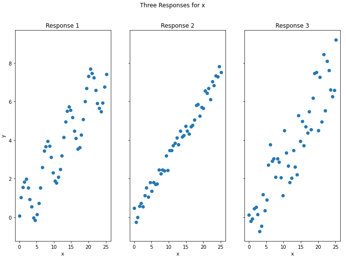
Each of these responses shows a linear trend from lower-left to upper-right. Let’s assume we have fitted a linear regression model to each of these responses. We can plot the model along with the data:
## plot the data ##
fig, axes = plt.subplots(1, 3, figsize=(12,8), sharey=True)
axes[0].scatter(x_true,y_true1)
axes[0].plot(x_true,y_pred,color='r')
axes[0].set_xlabel('x')
axes[0].set_ylabel('y')
axes[0].set_title('Response 1')
axes[1].scatter(x_true,y_true2)
axes[1].plot(x_true,y_pred,color='r')
axes[1].set_xlabel('x')
axes[1].set_title('Response 2')
axes[2].scatter(x_true,y_true3)
axes[2].plot(x_true,y_pred,color='r')
axes[2].set_xlabel('x')
axes[2].set_title('Response 3')
fig.suptitle('Three Responses for x Plus Linear Regression Fit')
fig.legend(['model','data'])
plt.show()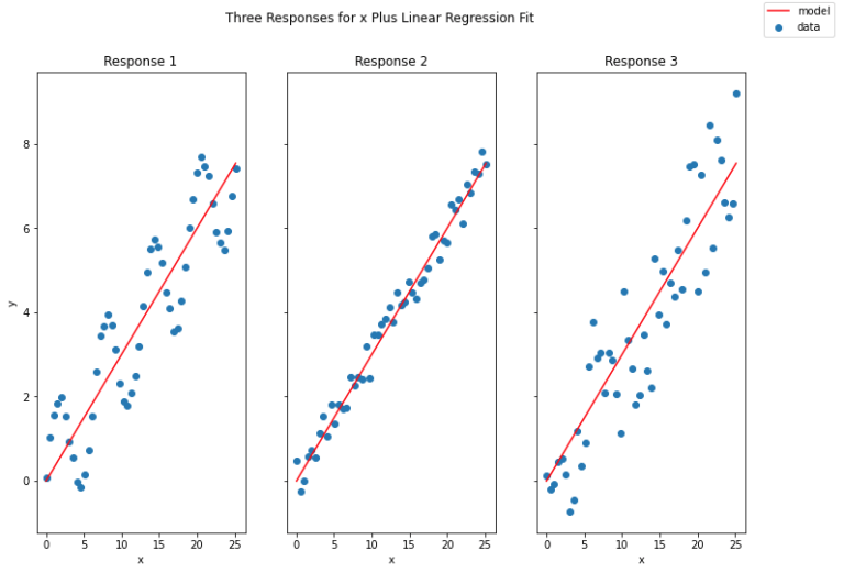
It’s clear that the model has captured the linear trend in each of the responses. However, the amount of variation in these data around the trend line is significantly different between the responses. We can measure the amount of variation in these data, that are explained by our model, by computing the coefficient of determination R^2. To do this, let’s make use of the function available from scikit-learn:
## compute the r2 score for each response ##
print("R2 score for Response 1: %.2f" % r2_score(y_true1,y_pred))
print("R2 score for Response 2: %.2f" % r2_score(y_true2,y_pred))
print("R2 score for Response 3: %.2f" % r2_score(y_true3,y_pred))
R2 score for Response 1: 0.79
R2 score for Response 2: 0.98
R2 score for Response 3: 0.82
Responses 1 & 3 show a similar R^2 score, whereas nearly all the variation in response 2 is explained by the linear model. This makes sense, as response 2 shows far less scatter around the trend line when compared with the other responses.
What can we say about responses 1 & 3? Response 3 shows much more noise when compared with response 2, however the pattern in these data is the same: a straight trend line. As such, the lower R^2 score here doesn’t indicate a bad model: it simply reflects the level of noise/uncertainty inherent in these data. Response 1 is different: it is apparent from the plot that superimposed on the trend is a sinusoidal component in these data. Therefore, the lower R^2 score here is due to a poor choice of model, as linear regression will not capture this aspect of the response.
This example illustrates that when using the coefficient of determination, it is always important to keep the context of the problem in mind. Acceptable values of R^2 in one discipline (i.e. the physical sciences) will be quite different to those in another (i.e. the social sciences). It is also always important to note how relevant a linear regression model is to the problem at hand: non-linear data should either be transformed into linear data, or be fitted with an appropriate alternative model.
Related Posts
Hi I'm Michael Attard, a Data Scientist with a background in Astrophysics. I enjoy helping others on their journey to learn more about machine learning, and how it can be applied in industry.