For this post, I will implement Linear Regression in Python from scratch. We will start with the fundamental assumptions and mathematical foundations, and work straight through to implementation in Python.  

Note: for those who prefer video content, you can watch me work through the content in this article by scrolling to the bottom of this post.

Motivation for Linear Regression

It is no secret that the past few years have seen a considerable rise in the interest in artificial intelligence and machine learning, much of it being fuelled by the developments in Deep Learning starting in the early 2000’s. This has caused simpler algorithms to be often overlooked by enthusiasts and beginners in the field.  However, for many practical applications it is these simple algorithms that often perform best, and are much more interpretable.  Here we’ll cover one of the simplest learning algorithms developed, linear regression. For any business application where a linear relationship exists between variables, this is a powerful technique for modelling the behaviour of the process, gaining insights, and generating predictions.

Initially developed in the early 19th by Adrien-Marie Legendre and Johann Carl Friedrich Gauss, linear regression is a statistical learning method by which a linear relationship is modelled between a response (y) and one or more independent variables (x).  The original formulation utilised the least squares estimation method, although other techniques have since been developed.  In the case of two or more independent variables, the algorithm is referred to as multiple linear regression.

Assumptions and Considerations

Here I will list the key assumptions behind the derivation of the linear regression algorithm: 

  • a linear model for continuous variables
  • the population of errors have a mean of zero
  • the independent variables are uncorrelated with the error
  • there should be zero autocorrelation in the error
  • the population of errors have constant variance
  • the independent variables are not linearly correlated with one another
  • the population of errors follows a normal distribution

Derivation of the Linear Regression Algorithm

Mathematically, a linear regression model assumes the following relationship between independent variables and response:

y_{i} = \beta_{0} + \beta_{1}x_{i,1} + \beta_{2}x_{i,2} + … + \beta_{N}x_{i,N} + \epsilon_{i}    (1)

Where the index i ranges over all available data points i=1…T. In its most general form, there are N+1 model parameters \beta_{0}, \beta_{1}, … \beta_{N} for N independent variables. The \epsilon_{i} term indicates the error between the response and the linear combination of independent variables.

Our objective is to find optimal values for the parameters \beta_{0}, \beta_{1}, … \beta_{N}. We can facilitate this by rewriting equation (1) in matrix notation by considering the following:

\bold{y} = \begin{bmatrix} y_1 \\ y_2 \\ . \\ . \\ . \\ y_T \end{bmatrix}, \bold{\beta} = \begin{bmatrix} \beta_0 \\ \beta_1 \\ . \\ . \\ . \\ \beta_N \end{bmatrix}, \bold{X} = \begin{bmatrix} 1 & x_{1,1} & … & x_{1,N} \\ 1 & x_{2,1} & … & x_{2,N} \\ … & … & … & … \\ … & … & … & … \\ 1 & x_{T,1} & … & x_{T,N} \end{bmatrix}, \bold{\epsilon} = \begin{bmatrix} \epsilon_1 \\ \epsilon_2 \\ . \\ . \\ . \\ \epsilon_T \end{bmatrix}    (2)

\bold{y} = \bold{X}\bold{\beta} + \bold{\epsilon}    (3)

Note that (3) represents a matrix equation which encompasses all the available data for calculating \beta.

To determine \beta we’ll need to specify a loss function to optimise.  Here we will take advantage of the sum of squares error SSE: 

SSE = \sum_{i=1}^{T} \epsilon_{i}^{2} = \bold{\epsilon}^{‘}\bold{\epsilon}    (4)

where the superscript indicates the transpose. Expanding out the matrix multiplication: 

\bold{\epsilon}^{‘}\bold{\epsilon} = (\bold{y} – \bold{X}\bold{\beta})^{‘}(\bold{y} – \bold{X}\bold{\beta})

= \bold{y}^{‘}\bold{y} – \bold{y}^{‘}\bold{X}\bold{\beta} – (\bold{X}\bold{\beta})^{‘}\bold{y} + (\bold{X}\bold{\beta})^{‘}\bold{X}\bold{\beta}

Now let’s look closer at the second and third terms.  Both consist of the same set of variables, and the multiplication products have the dimensions of (1 \times T)(T \times N+1)( N+1 \times 1) = ( 1  \times 1) and ( 1 \times N+1 )( N+1 \times T )( T \times 1 ) = ( 1 \times 1 ) for the second and third terms, respectively.  Since these are scalars, we can determine (\bold{X}\bold{\beta})^{‘}\bold{y} = \bold{y}^{‘}\bold{X}\bold{\beta}:

= \bold{y}^{‘}\bold{y} – 2(\bold{X}\bold{\beta})^{‘}\bold{y} + (\bold{X}\bold{\beta})^{‘}\bold{X}\bold{\beta}
= \bold{y}^{‘}\bold{y} – 2\bold{\beta}^{‘}\bold{X}^{‘}\bold{y} + \bold{\beta}^{‘}\bold{X}^{‘}\bold{X}\bold{\beta}

To find optimal values for \beta, we need to take the derivative of the loss function and set it to zero:

\frac{\partial SSE}{\partial \bold{\beta}} = – 2\bold{X}^{‘}\bold{y} + 2\bold{X}^{‘}\bold{X}\bold{\beta} = 0

\bold{\beta} = (\bold{X}^{‘}\bold{X})^{-1}\bold{X}^{‘}\bold{y}    (5)

Equation (5) provides an analytical solution to the problem of fitting the model to the available data, and is the aforementioned least squares estimation method. The appeal of an analytical solution is the computational efficiency by which the model parameters can be found (as opposed to using an iterative optimisation method).

Build and Test Linear Regression in Python

Will will begin our work by developing our own model, using the derivation outlined in the previous section.

Build a Custom Linear Regression Model

Let’s start by generating a small dataset with a single independent variable in Python.  To do this, first I’ll need to import a few packages that will be used throughout the examples: 

# imports
import numpy as np
import matplotlib.pyplot as plt
from sklearn.metrics import r2_score
from sklearn.datasets import make_regression

Now I will generate the data with a linear relationship between the independent variable (x) and the response (y), along with a error component (\epsilon) that follows a normal distribution:

# generate data
X,y,coef = make_regression(n_samples=200, 
                           n_features=1, 
                           n_informative=1, 
                           n_targets=1, 
                           bias=50, 
                           noise=15,
                           coef=True, 
                           random_state=42)
                           
# what is the true model coefficient?
coef
array(87.73730719)

In the code snippet above, I define the the number of samples (200) and the intercept term (50). Our model coefficient was determined within make_regression, however the value used is returned (87.74) along with the data.  The relationship between x, y, and \epsilon defined in the code above is:

y_i = 50 + 87.74\times x_i + \epsilon_i    (6)

where the error term is drawn from a normal distribution with mean 0 and standard deviation 15: \epsilon_i \sim N(0,15) , and the index i ranges over each sample.  Notice that equation (1) is just a generalisation of equation (6). 

Let’s visualise the data:

implement linear regression in python

Now I’ll construct a class that will encapsulate all the methods required for our linear regression model:

class LR(object):
    """
    Build a class to encompass linear regression with least squares estimation
    """
    
    def __init__(self) -> None:
        """
        Initialiser
        """
        # private parameters array
        self.__B = np.array([])
        
    def train(self, Xin: np.array, Yin: np.array) -> None:
        """
        Train function
        
        Inputs:
            Xin -> array of training predictor features
            Yin -> array of training labels
        """
        # add column of 1's to independent variables
        X        = np.ones((Xin.shape[0],Xin.shape[1]+1))
        X[:,1:]  = Xin
        # calculate the model parameters using least squares estimation
        Xfactors = np.matmul(np.linalg.inv(np.matmul(np.transpose(X),X)),np.transpose(X))
        self.__B   = np.matmul(Xfactors,Yin)
        
    def predict(self, Xin: np.array) -> np.array:
        """
        Predict function
        
        Inputs:
            Xin -> array of predictor features
            
        Outputs:
            Yp -> model predictions
        """
        # add column of 1's to independent variables
        X       = np.ones((Xin.shape[0],Xin.shape[1]+1))
        X[:,1:] = Xin
        # calculate predictions
        Yp      = np.matmul(X,self.__B)
        # return predictions
        return(Yp)
    
    def return_B(self) -> np.array:
        """
        Return model parameters
        
        Outputs:
            Array of learned model parameters
        """
        return(self.__B)

The class functions are as follows:

  • __init__(self) : this is the initialiser function which executes automatically when a class instance is declared. The model parameters are initialised here.
  • train(self,Xin,Yin) : calculates the model parameters according to equation (5), and stores the results internally.
  • predict(self,Xin) : predicts response values based upon the input Xin values, and the internally stored model parameters.
  • return_B(self) : return the model parameters.

With this class I’ll now declare an instance, fit the model to the data, and generate predictions:

# declare a LR object
lr = LR()
# fit the model
lr.train(X,y)
# make predictions
ypred = lr.predict(X)

Plotting the results:

implement linear regression in python

We can evaluate the model fit using the coefficient of determination (R^2) metric, which compares the variance in the data unexplained by the model, to the total variance in the data:

R^2 = 1 – \frac{\textrm{Unexplained} \quad \textrm{Variation}}{\textrm{Total} \quad \textrm{Variation}}    (7)

Seeing the above equation, it’s apparent that an ideal model will produce a R^2 value of 1.  So what value do we get for our model?

# what is our R2 score?
r2_score(y,ypred)
0.9662908496470797

This is quite a nice result, and shows that the model we built is working well.  Finally, let’s take a look at the learned parameters to see if we can recover the values we entered when creating the data:

# view our learned model parameters
lr.return_B()
array([52.14277085, 87.1809762 ])

Recall that the intercept and slope we specified, when creating these data, are 50 and 87.74, respectively.  This confirms our model is functioning well.

Another option to building our own model is to use the scikit-learn linear regression API: 

Scikit-Learn Linear Regression Model

First we’ll need to import this package:

# imports
from sklearn.linear_model import LinearRegression

Next let’s create an instance, fit the model to the data, and predict values:

# declare a LinearRegression object
lr = LinearRegression()
# fit the model
lr.fit(X,y)
# make predictions
ypred = lr.predict(X)

Similarly to the previous analysis, let’s plot the results, determine the R^2 value, and display the learned model parameters:

implement linear regression in python
# what is our R2 score?
lr.score(X,y)
0.9662908496470797
# view our model parameters
print(lr.intercept_)
print(lr.coef_)
52.142770851531786
[87.1809762]

We can see here that the results are virtually identical to those we obtained using our custom built class.

Final Remarks & Video

In this article you’ve learned:

  • The motivation behind the linear regression algorithm, and when it was developed
  • The derivation of linear regression, with least squares estimation
  • How to implement linear in Python from scratch
  • How to use the linear regression module provided by the popular scikit-learn library

For those who prefer video, I have covered the material in this article here:

I hope you enjoyed this article, and gained some value from it!  If you would like to take a closer look at the code presented here please take a look at my GitHub. If you have any questions or comments, please leave them below.

Related Posts

5 1 vote
Article Rating
Subscribe
Notify of
guest

3 Comments
Oldest
Newest Most Voted
Inline Feedbacks
View all comments
Efren Plata
Efren Plata
3 years ago

Congrats for your web page Mike, and thank you for recall me linear regression and least squares estimation method.

Abigail Plata
Abigail Plata
1 year ago

Thanks! Great information
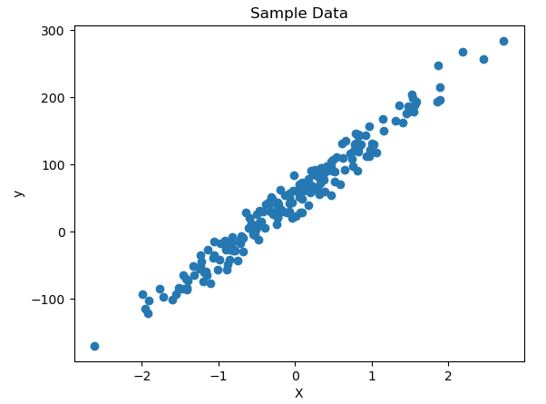
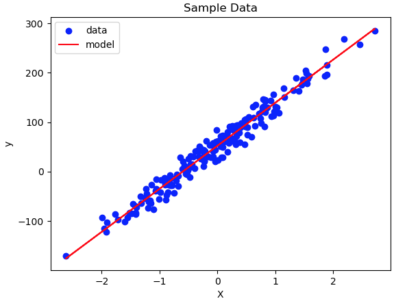
3
0
Would love your thoughts, please comment.x
()
x
Newsletter Signup