For this post, we will build a logistic regression classifier in Python. We will start from first principles, and work straight through to implementation in Python code. Performance of our implementation will then be tested against a small dataset. We will also compare these results with those that can be obtained with the logistic regression model available from scikit-learn.
Table of Contents
Note: for those who prefer video content, you can watch me work through the content in this article by scrolling to the bottom of this post.
Motivation to Build a Logistic Regression Classifier
The problem of predicting a categorical variable is generally termed as classification. Classification is an extensively studied and widely applicable branch of machine learning: tasks such as determining whether a given email is spam, to whether an image contains a dog or a cat, etc. all fall under this category. In this article we’ll cover one of the simplest classification algorithms, logistic regression.
The mathematical foundations for logistic regression were initially developed by Pierre François Verhulst and Adolphe Quetelet, during the 1830s to 1840s, in their work on population growth. The work of Joseph Berkson in the 1940s to 1950s saw the formal development of logistic regression for the case of a dependent variable with just 2 classes. The 1960s saw the development of the multinomial logistic regression model, where the dependent variable has more than 2 classes, with the work of David Cox & Henri Thiel.
Assumptions and Considerations to Build a Logistic Regression Classifier
Here I’ll list the key assumptions behind the the derivation that we’ll work though in the next section:
- the dependent variable is categorical in nature
- the independent variables are independent of, and uncorrelated with, each other
- there is a linear relationship between the independent variables and the log-odds of the dependent variable
- a sufficient sample size, such that each class in the dependent variable is well represented
- dependent variable classes are balanced
Derivation of Logistic Regression
For the sake of simplicity we will limit the derivation here to the case of a two-class problem, where the dependent variable (y) can take on only two values {0,1}. Note that because of this characteristic of y, it is not possible to use linear regression to model these data, since the output for this model is not bounded to {0,1}!
To build a model of this dataset, we will adopt a probabilistic approach. The probability for either class will be assumed to take on the form of the sigmoid or logistic function:
P(y_1|\bold{x}) = \frac{\exp(\beta_0 + \bold{\hat{\beta}}^T\bold{x})}{1 + \exp(\beta_0 + \bold{\hat{\beta}}^T\bold{x})} (1)
P(y_0|\bold{x}) = \frac{1}{1 + \exp(\beta_0 + \bold{\hat{\beta}}^T\bold{x})} (2)
where \bold{x} = \begin{bmatrix} x_1 \\ x_2 \\ . \\ . \\ . \\ x_M \end{bmatrix} is a vector of independent variables, \bold{\hat{\beta}} = \begin{bmatrix} \beta_1 \\ \beta_2 \\ . \\ . \\ . \\ \beta_M \end{bmatrix} is a vector of model parameters, \beta_0 is the model bias parameter, y_0 represents the case where y = 0, and y_1 represents the case where y = 1. To better understand these equations, we can plot both of them:
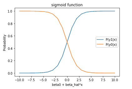
The model is constructed such that smaller values for \beta_0 + \hat{\beta}^T\bold{x} will favour the y = 0 case, while increasingly larger values will predict the y = 1 case. The goal for fitting the logistic regression model is to find the set of model parameters {\beta_0,\hat{\beta}} such that the output probability from equation (1) is close to 1.0 for cases where y = 1, and the output probability from equation (2) is close to 1.0 for cases where y = 0.
The plots of equations (1) and (2), along with paying close attention to the form of these equations, makes a few things apparent:
- P(y_1|\bold{x}) + P(y_0|\bold{x}) = 1
- As \bold{x} \rightarrow \infty then P(y_1|\bold{x}) \rightarrow 1 and P(y_0|\bold{x}) \rightarrow 0
- As \bold{x} \rightarrow -\infty then P(y_1|\bold{x}) \rightarrow 0 and P(y_0|\bold{x}) \rightarrow 1
Equations (1) and (2) have the properties of cumulative probability distribution functions. Output probabilities from these equations can be mapped to y by adhering to:
- P(y_1|\bold{x}) < 0.5 \implies y = 0 and P(y_1|\bold{x}) > 0.5 \implies y = 1
- P(y_0|\bold{x}) < 0.5 \implies y = 1 and P(y_0|\bold{x}) > 0.5 \implies y = 0
The decision boundary for this classifier is therefore at P(y_1|\bold{x}) = 0.5 and P(y_0|\bold{x}) = 0.5. To get a better intuition on this boundary, we can express (1) and (2) in terms of a odds ratio at the boundary:
\frac{P(y_1|\bold{x})}{P(y_0|\bold{x})} = \frac{0.5}{0.5} = 1
Taking the natural logarithm of both sides, and noting the forms of (1) and (2), we can write:
\ln(\frac{P(y_1|\bold{x})}{P(y_0|\bold{x})}) = \beta_0 + \hat{\beta}^T\bold{x} = 0 (3)
where \ln() is the natural logarithm. It is apparent from (3) that the decision boundary is linear for this model, along with the log-odds in general. We can also note that the log-odds are changed by \hat{\beta}^T for every unit change in \bold{x}.
We’ll now focus on actually fitting the model. Notice that (1) and (2) are exponential functions, and as such an analytic least squares estimation isn’t possible. Instead, we will fit the model parameters {\beta_0,\hat{\beta}} by maximum likelihood estimation (MLE), which is an iterative method. First let’s take note of the following:
- The exponent in the conditional probabilities (1) and (2) will be written as: \beta_0 + \hat{\beta}^T\bold{x} = \beta^T\bold{x}, where \beta includes {\beta_0,\hat{\beta}}, and \bold{x} on the right hand side includes a 1 as the first element
- To emphasise the dependence on the model parameters, we’ll set P(y_1|\bold{x}) = P_1(\bold{x};\beta) and P(y_0|\bold{x}) = P_0(\bold{x};\beta)
- Specific to the two-case problem, we can set P(y_1|\bold{x}) = P(\bold{x};\beta) and P(y_0|\bold{x}) = 1 – P(\bold{x};\beta)
The likelihood function is the probability of the data {\bold{x},y} given the model parameters (\beta). This is given by:
L(\bold{\beta}) = \prod_{i=1}^{N}P_{c_i}(\bold{x}_i;\beta)
where the index i iterates over all N data samples, and c_i can either be 0 or 1. The likelihood function is the product of N probabilities, and as such can be numerically unstable. For this reason, it’s more common to work with log-likelihood’s:
\ell(\beta) = \ln(L(\beta)) = \sum_{i=1}^{N}\ln(P_{c_i}(\bold{x}_i;\beta)) (4)
If we now make note of points 2 & 3 above, we can rewrite the terms within the summation as:
\ln(P_{c_i}(\bold{x}_i;\beta)) = y_i\ln(P(\bold{x}_i;\beta)) + (1-y_i)\ln(1-P(\bold{x}_i;\beta))
Therefore plugging the above result, equation (1), and equation (2) into (4) we get:
\ell(\beta) = \sum_{i=1}^N y_i\ln(P(\bold{x}_i;\beta)) + (1-y_i)\ln(1-P(\bold{x}_i;\beta))
= \sum_{i=1}^N y_i[\ln(\exp(\beta^T\bold{x}_i))-\ln(1 + \exp(\beta^T\bold{x}_i))] + (1-y_i)[-\ln(1+\exp(\beta^T\bold{x}_i))]
= \sum_{i=1}^N y_i\beta^T\bold{x}_i – \ln(1+\exp(\beta^T\bold{x}_i)) (5)
To maximise the log-likelihood we will calculate the first derivative of (5) with respect to \beta, and set it to zero:
\frac{\partial{\ell(\beta)}}{\partial\beta} = \sum_{i=1}^N y_i\bold{x}_i – \frac{1}{1+\exp(\beta^T\bold{x}_i)}\bold{x}_i\exp(\beta^T\bold{x}_i)
= \sum_{i=1}^N \bold{x}_i(y_i-P(\bold{x}_i;\beta)) = 0 (6)
Notice that \bold{x}_i is a column vector, and has such equation (6) represents M equations, which are non-linear in \beta. To solve (6), we’ll use the Newton-Raphson gradient ascent algorithm, which has the general form:
x_1 = x_0 – \frac{f(x_0)}{f^{'}(x_0)}
Applying this algorithm to equation (6) requires the second derivative of the log-likelihood:
\frac{\partial^2\ell(\beta)}{\partial\beta\partial\beta^T} = \sum_{i=1}^N -\bold{x}_i(\frac{\bold{x}_i^T\exp(\beta^T\bold{x}_i)}{1 + \exp(\beta^T\bold{x}_i)} – \frac{\exp(\beta^T\bold{x}_i)}{(1 + \exp(\beta^T\bold{x}_i))^2}\bold{x}_i^T\exp(\beta^T\bold{x}_i) )
= – \sum_{i=1}^N \bold{x}_i\bold{x}_i^T(P(\bold{x}_i;\beta) – P^2(\bold{x}_i;\beta))
= – \sum_{i=1}^N \bold{x}_i\bold{x}_i^TP(\bold{x}_i;\beta)(1 – P(\bold{x}_i;\beta)) (7)
Note here that the second derivative is negative, validating the concave nature of the likelihood function and ensuring the existence of a global maximum.
The Newton-Raphson algorithm for our purposes will be:
\beta^{'} = \beta – (\frac{\partial^2\ell(\beta)}{\partial\beta\partial\beta^T})^{-1}\frac{\partial\ell(\beta)}{\partial\beta} (8)
where \beta^{'} is the updated value for the model parameters at each iteration. To facilitate the calculation of \beta^{'} at each iteration step, let’s first rewrite equations (6) and (7) in matrix notation, and then plug the results into (8). Let’s start with the dependent and independent variables, along with the conditional probabilities:
\bold{y} = \begin{bmatrix} y_1 \\ y_2 \\ . \\ . \\ . \\ y_N \end{bmatrix}, \bold{X} = \begin{bmatrix} 1 & x_{1,1} & … & x_{1,M} \\ 1 & x_{2,1} & … & x_{2,M} \\ … & … & … & … \\ … & … & … & … \\ 1 & x_{N,1} & … & x_{N,M} \end{bmatrix}, \bold{P} = \begin{bmatrix} P(\bold{x}_1;\beta) \\ P(\bold{x}_2;\beta) \\ . \\ . \\ . \\ P(\bold{x}_N;\beta) \end{bmatrix} (9)
In addition we’ll set d_{i,i} = P(\bold{x}_i;\beta)(1 – P(\bold{x}_i;\beta)), and build a diagonal matrix such that:
\bold{D} = \begin{bmatrix} d_{1,1} & 0 & … & 0 \\ 0 & d_{2,2} & … & 0 \\ … & … & … & … \\ … & … & … & … \\ 0 & 0 & … & d_{N,N} \end{bmatrix} (10)
Therefore, using (9) and (10) we can express equations (6) and (7) as:
\frac{\partial{\ell(\beta)}}{\partial\beta} = \bold{X}^T(\bold{y}-\bold{P})
\frac{\partial^2\ell(\beta)}{\partial\beta\partial\beta^T} = -\bold{X}^T\bold{D}\bold{X}
and now write (8) in matrix notation:
\beta^{'} = \beta + (\bold{X}^T\bold{D}\bold{X})^{-1}\bold{X}^T(\bold{y}-\bold{P}) (11)
Equation (11) represents the update rule required to find the optimal set of model parameters, where all probabilities on the right hand side are calculated based on \beta. In practice, this update rule is executed until a certain tolerance threshold is reached, or a maximum number of iterations is completed.
Build and Test a Logistic Regression Classifier in Python
What we’ll work through below is the implementation of the model developed in the previous section. The model will be used to predict benign/malignant tumours in the scikit-learn breast cancer dataset.
Breast Cancer Dataset Exploration
Let’s start by importing the necessary libraries:
# imports
import numpy as np
import pandas as pd
import seaborn as sn
import matplotlib.pyplot as plt
from sklearn.datasets import load_breast_cancer
from sklearn.preprocessing import StandardScaler
from sklearn.model_selection import train_test_split
from sklearn.metrics import accuracy_score, precision_score, recall_score, roc_curve
and now proceed to load the dataset:
# load data
data = load_breast_cancer()
X    = data.data
y    = data.target
The matrix of independent variables \bold{X} consists of 30 features, while the label vector \bold{y} has elements that are either 1 for benign, and 0 for malignant.
We can now perform a train-test split on these data, where 20% will be reserved for testing:
# do train/test split
X_train, X_test, y_train, y_test = train_test_split(X, y, test_size=0.2, random_state=42, stratify=y)
Let’s take a look at our training labels, and check if the classes are balanced:
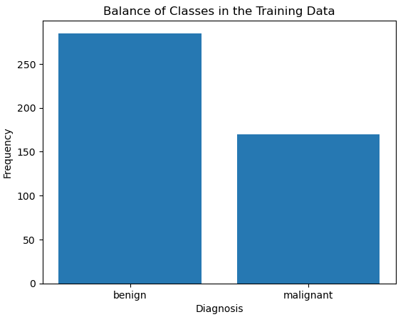
It’s evident that the classes are imbalanced. Let’s account for the difference by removing the excess benign cases, and adding these to the test data:
# work out relevant details for the dataset
idx_benign  = y_train == 1
n_benign    = np.sum(y_train)
n_malignant = y_train.shape[0] - n_benign
# split the training data according to the label
y_benign    = y_train[idx_benign]
y_malignant = y_train[~idx_benign]
X_benign    = X_train[idx_benign,:]
X_malignant = X_train[~idx_benign,:]
# workout the amount of excess
amount_excess = n_benign - n_malignant
# reform the training data
y_train = np.concatenate((y_malignant,y_benign[amount_excess:]),axis=0)
X_train = np.concatenate((X_malignant,X_benign[amount_excess:,:]),axis=0)
# add the excess to the test set
y_test = np.concatenate((y_test,y_benign[:amount_excess]),axis=0)
X_test = np.concatenate((X_test,X_benign[:amount_excess,:]),axis=0)
And so now if we repeat our bar plot of the label in the training data:
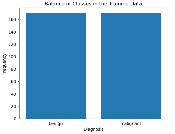
Now we can see that our class labels in the training data are balanced. Let’s now proceed to explore the independent variables/input features. I’ll generate a box plot to get a sense of the distributions and scales in the data. In addition, I will also produce a correlation heat map to determine what, if any, features are highly correlated:
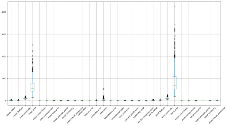
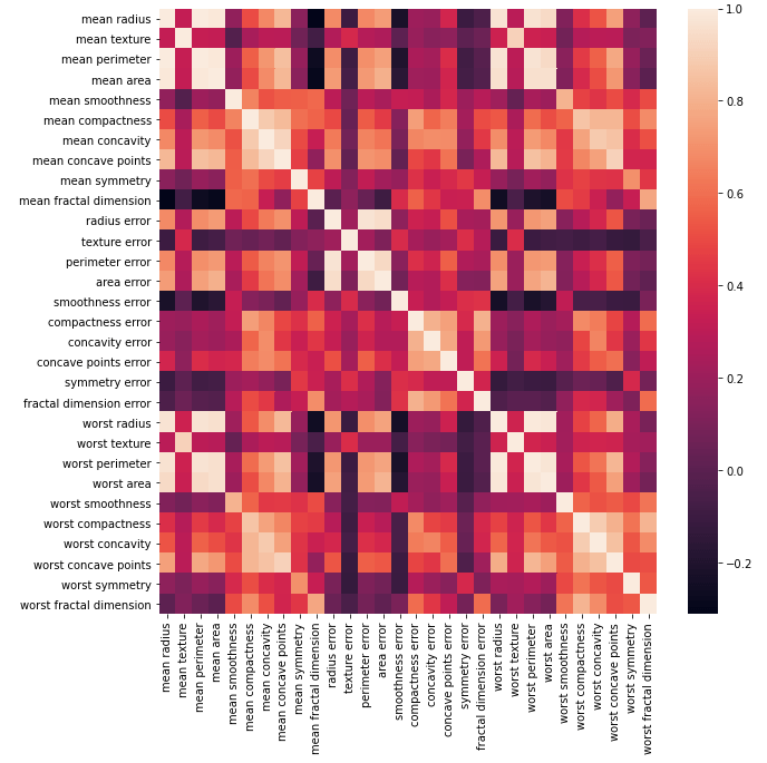
Note that the heat map was generated with Pearson correlation values, which measures linear correlations between variables. We can conclude from these plots that some features:
- have very different scales
- have skewed distributions
- are highly correlated
Highly correlated features should be removed from the dataset prior to modelling. Let’s take advantage of the build-in functions included in Pandas dataframes to indicate what features share a correlation coefficient > 0.8:
#package the independent variables into a dataframe
dfX_train = pd.DataFrame(X_train,columns=data.feature_names)
dfX_test = pd.DataFrame(X_test,columns=data.feature_names)
#compute the pearson correlation coefficients
dfCorr = dfX_train.corr()
# determine all feature combinations with corelation coef > 0.8
dfCorr     = dfCorr[dfCorr > 0.8].stack().reset_index()
dfCorr     = dfCorr[dfCorr.level_0!=dfCorr.level_1]
sCorrCount = dfCorr.groupby('level_0')['level_1'].agg(lambda x: set(x))
We can now print out the results:
# view results
sCorrCount
area error {worst area, perimeter error, radius error, me...
compactness error {concavity error, fractal dimension error}
concavity error {compactness error}
fractal dimension error {compactness error}
mean area {mean concave points, mean radius, area error,...
mean compactness {worst concavity, worst concave points, mean c...
mean concave points {worst concave points, mean radius, mean compa...
mean concavity {worst concavity, worst concave points, mean c...
mean perimeter {mean concave points, mean radius, mean area, ...
mean radius {mean concave points, mean perimeter, mean are...
mean smoothness {worst smoothness}
mean texture {worst texture}
perimeter error {area error, radius error}
radius error {area error, perimeter error}
worst area {mean concave points, mean radius, area error,...
worst compactness {worst concavity, worst concave points, mean c...
worst concave points {worst concavity, mean concave points, worst c...
worst concavity {worst concave points, mean concavity, mean co...
worst fractal dimension {worst compactness}
worst perimeter {worst concave points, mean concave points, me...
worst radius {mean concave points, mean radius, mean perime...
worst smoothness {mean smoothness}
worst texture {mean texture} We can see that there are quite a few highly correlated features. Let’s now determine a list of correlated features we can remove from the data, and proceed to remove them:
# determine complete list of correlated features
corr_features = set()
for features in sCorrCount:
    corr_features = corr_features | features

# determine list of correlated features to remove
to_remove = set()
for keep, remove in sCorrCount.items():
    # check if we should add to our remove list?
    if corr_features and (keep not in to_remove):
        # add to list of features to remove
        to_remove = to_remove | remove
        # update corr_features
        corr_features = corr_features - remove

# drop correlated features
dfX_train.drop(list(to_remove), axis=1, inplace=True)
dfX_test.drop(list(to_remove), axis=1, inplace=True)
Let’s now make a box plot of the truncated dfX_train:
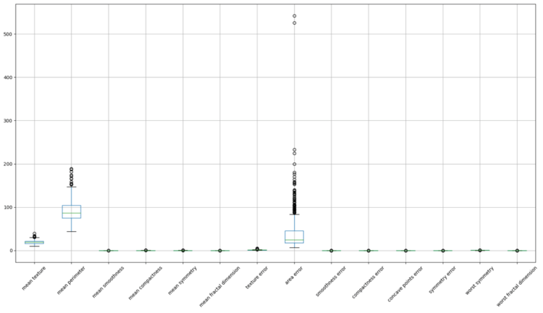
The remaining features still have variations in terms of scale and distribution. To facilitate the operation of the learning algorithm, we should scale these features such that each has a mean of zero and standard deviation of 1. This ensures that the gradients used during the optimisation are influenced by each feature equally. We’ll use the scikit-learn StandardScaler to accomplish this:
# scale input features
scaler  = StandardScaler()
X_train = scaler.fit_transform(dfX_train)
X_test  = scaler.transform(dfX_test)
Build a Custom Logistic Regression Classifier
Now let’s encapsulate the algorithm, derived in the previous section, into a Python class:
class LogR(object):
    """
    Class to encompass the logistic regression model with the Newton-Raphson algorithm
    """

    def __init__(self, max_iter: int=100, tol: float=1e-4) -> None:
        """
        Initialiser function for a class instance

        Inputs:
            max_iter      -> maximum number of iterations of the Newton-Raphson algorithm
            tol           -> tolerance threshold to terminate the Newton-Raphson algorithm
        """
        self.__B        = np.array([])
        self.__max_iter = max_iter
        self.__tol      = tol

    def train(self, Xin: np.array, Yin: np.array) -> None:
        """
        Training function for a class instance

        Inputs:
            Xin -> training set of predictor features
            Yin -> training set of associated labels
        """
        # add column of 1's to independent variables
        X       = np.ones((Xin.shape[0],Xin.shape[1]+1))
        X[:,1:] = Xin
        # ensure correct dimensions for the input labels
        Y = Yin.reshape(-1,1)
        # prepare parameters array
        self.__B = np.zeros((X.shape[1],1))
        # loop through the Newton-Raphson algorithm
        for _ in range(self.__max_iter):
            # compute conditional probabilities
            P = 1/(1 + np.exp(-np.matmul(X,self.__B)))
            # built diagonal matrix
            D = np.diag(np.multiply(P,(1-P)).flatten())
            # parameter update rule
            Minv      = np.linalg.inv(np.matmul(np.matmul(X.T,D),X))
            dB        = np.matmul(np.matmul(Minv,X.T),np.subtract(Y,P))
            self.__B += dB
            # check if we've reached the tolerance
            if self.__tol > np.linalg.norm(dB):
                break

    def predict(self, Xin: np.array, return_prob: bool=False) -> np.array:
        """
        Predict function for a class instance

        Inputs:
            Xin         -> input predictor features
            return_prob -> boolean to determine if probability or label is returned
        Outputs:
            numpy array of model predictions for the Xin inputs
        """
        # add column of 1's to independent variables
        X       = np.ones((Xin.shape[0],Xin.shape[1]+1))
        X[:,1:] = Xin
        # calculate predictions
        Yp      = 1/(1 + np.exp(-np.matmul(X,self.__B)))
        # return predictions
        if not return_prob:
            Yp = Yp.round(decimals=0)
        return(Yp)

    def return_B(self) -> np.array:
        """
        Function to return model parameters

        Output:
            self.__B -> array of learned model parameters
        """
        return(self.__B)
The class functions are as follows:
- __init__(self, max_iter=100, tol=1e-4) : this is the initialiser function which executes automatically when a class instance is declared. The model parameters are initialised here. max_iter is the maximum number of iterations to carry out, and tol is the tolerance on which to halt the learning procedure (before max_iter is reached).
- train(self, Xin, Yin) : this function calculates the model parameters according to equation (11), and stores the results internally. The training data is composed of input independent variables Xin, and associated labels, Yin.
- predict(self, Xin, return_prob=False) : this function predicts response values based upon the input Xin values, and the internally stored model parameters. If return_prob is set to True, the probabilities for y = 1 are returned instead of the actual label values.
- return_B(self) : return the model parameters
We can now declare a class instance, train it, and predict the labels on the test set along with their associated probabilities:
# fit our logistic regression model & generate predictions
lr    = LogR()
lr.train(X_train,y_train)
ypred = lr.predict(X_test)
yprob = lr.predict(X_test,return_prob=True)
In order to determine how well our model is doing, we will calculate the accuracy, precision, and recall of the results. All of these metrics range from [0,1], where 0 and 1 are the worst and best possible results, respectively. We can use the functions imported from scikit-learn to measure these metrics:
# evaluate model performance
print("accuracy: %.2f" % accuracy_score(y_test,ypred))
print("precision: %.2f" % precision_score(y_test,ypred))
print("recall: %.2f" % recall_score(y_test,ypred))
accuracy: 0.90 precision: 0.99 recall: 0.89
These results indicate our model is functioning well with this data set. Finally, we can visualise the results by creating a Receiver Operating Characteristic (ROC) plot. This plot shows the False Positive Rate versus the True Positive Rate, for all possible decision rules (in our code of the LogLR class, the decision rule is set at 0.5). We can use the roc_curve function from scikit-learn to produce this plot:
# create a ROC plot
fpr,tpr,_ = roc_curve(y_test, yprob)
plt.plot(fpr,tpr)
plt.title('Receiver Operating Characteristic')
plt.plot([0, 1], ls="--")
plt.plot([0, 0], [1, 0] , c=".8"), plt.plot([1, 1] , c=".8")
plt.ylabel('True Positive Rate')
plt.xlabel('False Positive Rate')
plt.show()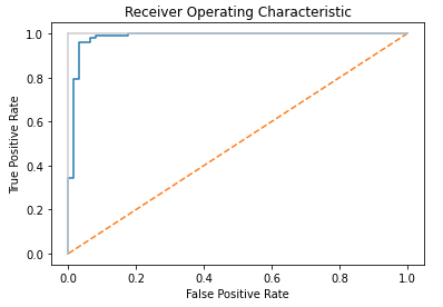
The diagonal orange line indicates the result for predictions made at random; the further our model results are from this line, and towards the upper left, the better the classifier correctly identifies true and false positives. This plot confirms what our earlier accuracy and precision calculations showed: the model functions as a reasonably good classifier for the breast cancer dataset used in this example.
Scikit-Learn Logistic Regression Model
Instead of building our own logistic regression model from scratch, it’s also possible to use the one available through scikit-learn:
# imports
from sklearn.linear_model import LogisticRegression
We can now train and predict using this model and the same data set as used previously:
# fit our data and generate predictions
lr    = LogisticRegression(penalty=None)
lr.fit(X_train,y_train)
ypred = lr.predict(X_test)
yprob = lr.predict_proba(X_test)

# evaluate model performance
print("accuracy: %.2f" % accuracy_score(y_test,ypred))
print("precision: %.2f" % precision_score(y_test,ypred))
print("recall: %.2f" % recall_score(y_test,ypred))
accuracy: 0.90 precision: 0.99 recall: 0.89
Finally we can also reproduce the ROC plot for these data:
# create a ROC plot
fpr,tpr,_ = roc_curve(y_test, yprob[:,1])
plt.plot(fpr,tpr)
plt.title('Receiver Operating Characteristic')
plt.plot([0, 1], ls="--")
plt.plot([0, 0], [1, 0] , c=".8"), plt.plot([1, 1] , c=".8")
plt.ylabel('True Positive Rate')
plt.xlabel('False Positive Rate')
plt.show()
We can see that the accuracy, precision, and recall metrics, along with the ROC plot, are exactly the same to the results obtained with our custom built model.
Final Remarks & Video
In this article you’ve learned:
- The motivation behind logistic regression and when it was developed
- How logistic regression with maximum likelihood estimation is derived
- How to build a logistic regression classifier in Python
- How to use the logistic regression module provided by the popular scikit-learn library
If you like video content, I have also produced a YouTube tutorial covering the material discussed in this article:
I hope you enjoyed this article and gained some value from it! If you would like to take a closer look at the code presented here please take a look at my GitHub. If you have any questions or comments, please leave your remarks in the comments section below.
Related Posts
Hi I'm Michael Attard, a Data Scientist with a background in Astrophysics. I enjoy helping others on their journey to learn more about machine learning, and how it can be applied in industry.
Congratulations on building your website. Keep up the good work!
Thank you!
[…] I perform logistic regression to the output from step 2, to yield a predictive model for our […]