In this article, we will build a bagging classifier in Python from the ground-up. Our custom implementation will then be tested for expected behaviour. Through this exercise it is hoped that you will gain a deep intuition for how bagging works.
Table of Contents
Motivation to Build a Bagging Classifier
We saw in a previous post that the bootstrap method was developed as a statistical technique for estimating uncertainty in our models. Here we will extend this technique by taking advantage of our bootstrap samples to improve the quality of model predictions. This technique is called bootstrap aggregating, or bagging.
Bagging is an ensemble algorithm, in that multiple models are combined to produce a net result that outperforms any of the individual models. This approach can significantly reduce the amount of variance in the prediction results.
Bagging was first developed in 1994 by Breiman et al1. This paper demonstrated the accuracy improvements possible with classification and regression decision Trees, as well as with linear regression.
Bagging Assumptions and Considerations
It is essential that good bootstrap samples are obtained for bagging to work. As such, the assumptions from the bootstrap post still hold here.
Bagging works well in situations where perturbations in the data can cause significant differences in an individual model trained on these data. In this situation, bagging will lower the variance and prevent over fitting.
Although any model could be used in bagging, normally only rather simple models, that only perform moderately above that of random guessing, are used. These are termed weak learners.
Derivation of the Bagging Algorithm
The description here is an extension of the one given in the bootstrap post. We can take that we have already generated N bootstrap samples from the available training dataset. We should also have a separate set of predictors – input data for the actual values we want predictions for. These can come from a test set, or from live input in a production setting.
Our methodology is then as follows:
- Obtain a labelled training data set, as well as a set of independent variables for the predictions we want.
- Produce N bootstrap samples on the training data
- Loop through each of the i=1..N bootstrap samples:
- Fit a model to sample i
- Produce the desired predictions with this model. It is also possible to compute the standard error of the predictions using the out-of-bag samples
- Repeat the above two steps, storing the trained models and predictions
- Aggregate the predictions. In the event of having a labelled test set, compare these results with the test dataset labels
- If the results from points 3 & 4 above are good, we can deploy our trained ensemble. Input data is provided to the ensemble, and each constituent model produces predictions. These predictions are aggregated to yield a final result
For the case where a train-test split was done on the labelled data, the methodology is illustrated below:
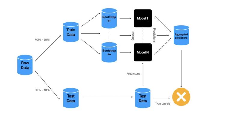
Different datasets are indicated in blue, while individual models are in black. Assessment of the ensemble performance is done at the decision node in orange. This assessment is done solely using the test dataset.
Normally anywhere between 70% – 90% of the available data are used for training, while the remainder are allocated to the test data set.
The aggregation of the ensemble predictions is normally done by computing the mean in the case of regression, while the mode can be used for classification.
Build a Bagging Classifier in Python
Disclaimer: re-running the below sections could result is slightly different results. This is a result of the random nature of the processes involved.
We can start this section by importing the required packages:
## imports ##
import numpy as np
from sklearn.base import clone
from sklearn.datasets import load_breast_cancer
from sklearn.model_selection import StratifiedKFold,cross_validate
from sklearn.tree import DecisionTreeClassifier
from sklearn.metrics import accuracy_score,precision_score,recall_score
Custom Bagging Tree Classifier
I will now build a class to encapsulate the functionality required for our bagging ensemble. To generate the bootstrap samples, I will make use of a modified version of the make_bootstraps function we built in the bootstrap post. As we’ll be investigating a classification dataset, the weak learner we will use here, to build our ensemble, is the decision tree classifier.
## make an ensemble classifier based on decision trees ##
class BaggedTreeClassifier(object):
    #initializer
    def __init__(self,n_elements=100):
        self.n_elements = n_elements
        self.models     = []

    #destructor
    def __del__(self):
        del self.n_elements
        del self.models

    #private function to make bootstrap samples
    def __make_bootstraps(self,data):
        #initialize output dictionary & unique value count
        dc   = {}
        unip = 0
        #get sample size
        b_size = data.shape[0]
        #get list of row indexes
        idx = [i for i in range(b_size)]
        #loop through the required number of bootstraps
        for b in range(self.n_elements):
            #obtain boostrap samples with replacement
            sidx   = np.random.choice(idx,replace=True,size=b_size)
            b_samp = data[sidx,:]
            #compute number of unique values contained in the bootstrap sample
            unip  += len(set(sidx))
            #obtain out-of-bag samples for the current b
            oidx   = list(set(idx) - set(sidx))
            o_samp = np.array([])
            if oidx:
                o_samp = data[oidx,:]
            #store results
            dc['boot_'+str(b)] = {'boot':b_samp,'test':o_samp}
        #return the bootstrap results
        return(dc)
Here the class is defined, and private member functions are implemented as follows:
- __init__(self,n_elements=100) : this is the initialiser function which executes automatically when a class instance is declared. The model parameters are initialised here. There is a single input argument, n_element, which defines how many models should be included in the ensemble.
- __del__(self) : this function is executed automatically when a class instance is destroyed. Class member variables are deleted here.
- __make_boostraps(self, data) : this function generates bootstrap samples on the input data array.
Let’s now define public functions for training the ensemble, and generating predictions with it:
#public function to return model parameters
    def get_params(self, deep = False):
        return {'n_elements':self.n_elements}

    #train the ensemble
    def fit(self,X_train,y_train,print_metrics=False):
        #package the input data
        training_data = np.concatenate((X_train,y_train.reshape(-1,1)),axis=1)
        #make bootstrap samples
        dcBoot = self.__make_bootstraps(training_data)
        #initialise metric arrays
        accs = np.array([])
        pres = np.array([])
        recs = np.array([])
        #iterate through each bootstrap sample & fit a model ##
        cls = DecisionTreeClassifier(class_weight='balanced')
        for b in dcBoot:
            #make a clone of the model
            model = clone(cls)
            #fit a decision tree classifier to the current sample
            model.fit(dcBoot[b]['boot'][:,:-1],dcBoot[b]['boot'][:,-1].reshape(-1, 1))
            #append the fitted model
            self.models.append(model)
            #compute the predictions on the out-of-bag test set & compute metrics
            if dcBoot[b]['test'].size:
                yp  = model.predict(dcBoot[b]['test'][:,:-1])
                acc = accuracy_score(dcBoot[b]['test'][:,-1],yp)
                pre = precision_score(dcBoot[b]['test'][:,-1],yp)
                rec = recall_score(dcBoot[b]['test'][:,-1],yp)
                #store the error metrics
                accs = np.concatenate((accs,acc.flatten()))
                pres = np.concatenate((pres,pre.flatten()))
                recs = np.concatenate((recs,rec.flatten()))
        #compute standard errors for error metrics
        if print_metrics:
            print("Standard error in accuracy: %.2f" % np.std(accs))
            print("Standard error in precision: %.2f" % np.std(pres))
            print("Standard error in recall: %.2f" % np.std(recs))

    #predict from the ensemble
    def predict(self,X):
        #check we've fit the ensemble
        if not self.models:
            print('You must train the ensemble before making predictions!')
            return(None)
        #loop through each fitted model
        predictions = []
        for m in self.models:
            #make predictions on the input X
            yp = m.predict(X)
            #append predictions to storage list
            predictions.append(yp.reshape(-1,1))
        #compute the ensemble prediction
        ypred = np.round(np.mean(np.concatenate(predictions,axis=1),axis=1)).astype(int)
        #return the prediction
        return(ypred)
- get_params(self,deep=False) : this function returns the input model parameters, and is only included here so that we can make use of scikit-learns cross-validation functionality.
- fit(self,X_train,y_train,print_metrics=False) : this function trains the ensemble using the provided arrays of predictors, X_train, and labels, y_train. If the print_metrics argument is set to True, the out-of-bag samples will be used to compute the standard error on our evaluation metrics. Note however that these data are unbalanced, and as such we will have to address this fact while modelling (Each individual decision tree classifier has been set with class_weight = ‘balanced’ for just this reason).
- predict(self,X) : this function produces predictions from the trained ensemble using the input X array of predictors.
We can now proceed to load in the data set. Here we use the same breast cancer data set previously analysed in the logistic regression & decision tree posts. As such, I will not do any data exploration here.
## load classification dataset ##
data = load_breast_cancer()
X    = data.data
y    = data.target
An instance of our ensemble class can now be made and trained. To reveal the standard errors in our evaluation metrics, I’ve set the print_metrics argument to True:
## declare an ensemble instance with default parameters ##
ens = BaggedTreeClassifier()

## train the ensemble & view estimates for prediction error ##
ens.fit(X,y,print_metrics=True)
Standard error in accuracy: 0.02
Standard error in precision: 0.02
Standard error in recall: 0.02
To measure the performance of the ensemble classifier, I am making use of the accuracy, precision, and recall metrics:
Accuracy = \frac{TP + TN}{TP + FP + TN + FN} (1)
Precision = \frac{TP}{TP + FP} (2)
Recall = \frac{TP}{TP + FN} (3)
where TP, TN, FP, FN are the counts of True Positives, True Negatives, False Positives, and False Negatives, respectively. We can make use of the functions provided by scikit-learn to calculate (1), (2), and (3).
The standard errors computed with our fit method gives us a measure for the expected prediction error using this ensemble. The results shown above look quite reasonable for the problem at hand.
Let’s now measure the performance of our ensemble! However instead of doing a simple train-test split, we will be using k-fold cross validation. This involves making a series of train-test splits on the data, and evaluating the ensemble on each partition. The results from each evaluation can then be combined to yield measurements that are less sensitive to any specific splitting of the data. Luckily, scikit-learn provides a function to take care of most of the work for us:
## use k fold cross validation to measure performance ##
scoring_metrics = ['accuracy','precision','recall']
dcScores        = cross_validate(ens,X,y,cv=StratifiedKFold(10),scoring=scoring_metrics)
print('Mean Accuracy: %.2f' % np.mean(dcScores['test_accuracy']))
print('Mean Precision: %.2f' % np.mean(dcScores['test_precision']))
print('Mean Recall: %.2f' % np.mean(dcScores['test_recall']))
accuracy: 0.96
precision: 0.96
recall: 0.97
We can see that 10 folds were included in our cross-validation analysis. The StratifiedKFold function ensures that each partition of the dataset has an equal ratio of the two classes in it. This is an additional treatment for unbalanced datasets.
These results look good, they represent an improvement, in terms of accuracy and recall, over the lone decision tree classifier (see classification results from the decision tree post). It is important to note that no hyperparameter tuning was done for the decision trees in our ensemble: further improvements to our ensemble are therefore possible (try it out!).
Scikit-Learn Bagging Tree Classifier
Let’s compare how our custom-built ensemble compares to the one available through scikit-learn:
## import the scikit-learn model ##
from sklearn.ensemble import BaggingClassifier

## declare a bagging classifier instance ##
ens = BaggingClassifier(base_estimator=DecisionTreeClassifier(class_weight='balanced'),n_estimators=100)

## use k fold cross validation to measure performance ##
scoring_metrics = ['accuracy','precision','recall']
dcScores        = cross_validate(ens,X,y,cv=StratifiedKFold(10),scoring=scoring_metrics)
print('Mean Accuracy: %.2f' % np.mean(dcScores['test_accuracy']))
print('Mean Precision: %.2f' % np.mean(dcScores['test_precision']))
print('Mean Recall: %.2f' % np.mean(dcScores['test_recall']))
accuracy: 0.96
precision: 0.97
recall: 0.97
The results here are very similar with those obtained with our custom ensemble classifier. The difference between the two falls within the range of the standard errors computed earlier in this section. Note that the default base model for the scikit-learn ensemble is a decision tree classifier. This can be changed by the engineer if desired.
Final Remarks
In this article you’ve learned:
- The motivation behind bagging ensembles, and when this approach was developed
- The algorithmic basis behind bagging ensembles
- How to build a bagging classifier in Python
- How to use the bagging classifier functionality provided by the popular scikit-learn library
I hope you enjoyed this article and gained some value from it! If you would like to take a closer look at the code presented here please take a look at my GitHub.
Related Posts
Addendum
- Breiman, Leo. 1994. Bagging Predictors, Department of Statistics, UC Berkeley. Technical Report No. 421.
Hi I'm Michael Attard, a Data Scientist with a background in Astrophysics. I enjoy helping others on their journey to learn more about machine learning, and how it can be applied in industry.