Introduction
Machine learning models are developed primarily to produce good predictions for some desired quantity. What we want is a model that can generalise well the patterns in our data in order to make reasonable predictions. Two important measures of how well a model generalises are bias and variance:
- Bias is the tendency for a model to make predictions that deviate from the true values in a consistent way. A model with high bias lacks some expressive ability to simulate the process in question, and is said to underfit the data
- Variance is the effect of a model that is too sensitive to noise present in the data. A model with high variance has too much expressive ability for the process in question, and is said to overfit the data
For the situation where we have data (x,y) and a model that makes predictions \hat{y}(x), the bias and variance are given by:
Bias = E(\hat{y}(x)) – y (1)
Variance = E([E(\hat{y}(x)) – \hat{y}(x)]^2) (2)
where the E(x) represents the expected value of x. Making a machine learning model that generalises well is typically a task of balancing the amount of bias and variance present, since high bias implies low variance, and vice versa.
We can examine these concepts further through example.
Python Coding Example
Let’s start here by importing the necessary packages, and then generate some toy data:
## imports ##
import numpy as np
import matplotlib.pyplot as plt

## generate some data ##
x_true = np.linspace(0,8*np.pi,50)
y_true = np.sin(x_true) + 0.3*x_true + 0.3*np.random.rand(x_true.shape[0])
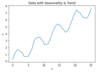
We can now plot these data to visualise the relationship between x and y:
## plot the data ##
plt.plot(x_true,y_true)
plt.title('Data with Seasonality & Trend')
plt.xlabel('x')
plt.ylabel('y')
plt.show()
We can see that these data have two principal components: a trend of y increasing with x, and a seasonal variation comprising 4 cycles in total.
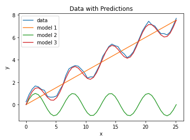
Now let’s assume we have 3 different models that we fit to the data. Plotting these models with the raw data reveals:
## plot the data with predictions ##
plt.plot(x_true,y_true)
plt.plot(x_true,y_pred1)
plt.plot(x_true,y_pred2)
plt.plot(x_true,y_pred3)
plt.title('Data with Predictions')
plt.xlabel('x')
plt.ylabel('y')
plt.legend(['data','model 1','model 2','model 3'])
plt.show()

It’s apparent that models 1 & 2 do not fit the data very well: model 1 captures the trend but fails with mimicking the seasonal component. Model 2 captures the seasonality but fails to reproduce the trend. Both of these models are said to have high bias. This situation can arise by choosing an inadequate model (linear regression in the case of model 1, a simple sine function for model 2), or by having insufficient training data for the problem at hand. Model 3 follows the data well, and thus generalises the data generating process in a satisfactory way.
Let’s continue by generating some additional data:
## generate some data ##
x_true = np.linspace(0,25,50)
y_true = 0.3*x_true + 2*np.random.rand(x_true.shape[0])

## plot the data ##
plt.scatter(x_true,y_true)
plt.title('Data with trend')
plt.xlabel('x')
plt.ylabel('y')
plt.show()
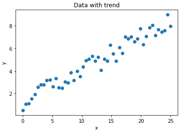
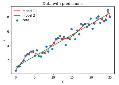
We can see that these data follow a linear trend, but there’s a fair amount of noise. Now let’s fit two different models to these data, and plot the results:
## plot the data with predictions ##
plt.scatter(x_true,y_true)
plt.plot(x_true,y_pred1,color='r')
plt.plot(x_true,y_pred2,color='g')
plt.title('Data with predictions')
plt.xlabel('x')
plt.ylabel('y')
plt.legend(['model 1','model 2','data'])
plt.show()

Model 1 shows quite a lot of variation, as it attempts to fit the noise in the data. This model is said to have high variance, and this can result from using a model with too much expressive ability (in this case, a 20-degree polynomial). Model 2 is far simpler, and generalises the trend in the data very well.
Related Posts
Hi I'm Michael Attard, a Data Scientist with a background in Astrophysics. I enjoy helping others on their journey to learn more about machine learning, and how it can be applied in industry.

[…] can arise in the event of overfitting. In this scenario, the sample sizes at each node can become small enough to effect the training […]
[…] algorithm. One of the main considerations listed in that post is that these models are prone to overfitting. In fact, this is one of the main disadvantages of Decision Trees. This is because the CART […]
[…] over a subsample of the training data. Outliers can start to have a bigger impact if the tree has overfitted. This topic was covered in a previous […]