Overfitting is a common problem with Decision Trees. Pruning consists of a set of techniques that can be used to simplify a Decision Tree, and enable it to generalise better. Pruning Decision Trees falls into 2 general forms: Pre-Pruning and Post-Pruning. Both will be covered in this article, using examples in Python.
Table of Contents
What is Pruning a Decision Tree?
In a previous article, I covered in detail the CART Decision Tree algorithm. One of the main considerations listed in that post is that these models are prone to overfitting. In fact, this is one of the main disadvantages of Decision Trees. This is because the CART learning algorithm will, if unrestricted, tend to continue branching until the training set is perfectly fitted.
Pruning involves simplifying the tree structure, and in effect regularises the model. While this simpler model will tend to have a higher training error, it will generalise far better on unseen data. There are 2 categories of Pruning Decision Trees:
- Pre-Pruning: this approach involves stopping the tree before it has completed fitting the training set. Pre-Pruning involves setting the model hyperparameters that control how large the tree can grow.
- Post-Pruning: here the tree is allowed to fit the training data perfectly, and subsequently it is truncated according to some criteria. The truncated tree is a simplified version of the original, with the least relevant branches having been removed.
Python Examples
Let’s work through a few examples to illustrate overfitting, Pre-Pruning, and Post-Pruning with Decision Trees. I will make use of the Iris dataset for the purpose of these examples. We can begin by making the necessary package imports, and then load in our dataset:
# imports
import numpy as np
from sklearn.tree import DecisionTreeClassifier, plot_tree
from sklearn.model_selection import train_test_split
from sklearn.datasets import load_iris
import matplotlib.pyplot as plt
from sklearn.metrics import classification_report
from sklearn.model_selection import GridSearchCV, RandomizedSearchCV
from scipy.stats import uniform, poisson

# load in the data
data = load_iris()

# isolate out the data we need
X             = data.data
y             = data.target
class_names   = data.target_names
feature_names = data.feature_names
Next let’s do a stratified train-test split on these data:
# perform a train-test split
X_train, X_test, y_train, y_test = train_test_split(X, y, test_size=0.2, random_state=42, stratify=y)
Overfitting a Decision Tree
To see why Pruning is needed, let’s first investigate what happens to a Decision Tree with no limits to growth. As such, we can train a Decision Tree classifier on the Iris data with default hyperparameter values:
# fit a decision tree classifier
clf = DecisionTreeClassifier(random_state=42)
clf.fit(X_train,y_train)
The structure of the learned model can be easily visualised with scikit-learn’s plot_tree:
# visualise the decision tree
fig = plt.figure(figsize=(16,8))
_ = plot_tree(clf,
              feature_names=feature_names,
              filled=True,
              class_names=class_names,
              fontsize=10)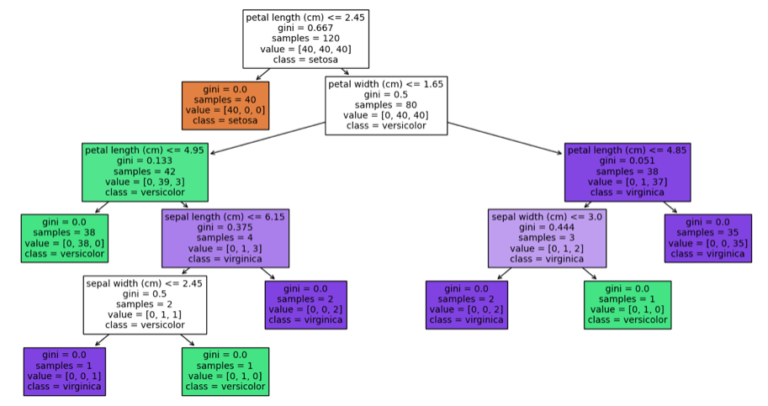
To measure performance, let’s put together a classification report on the test set:
# produce classification report
y_pred = clf.predict(X_test)
print(classification_report(y_test, y_pred))
precision recall f1-score support
0 1.00 1.00 1.00 10
1 0.90 0.90 0.90 10
2 0.90 0.90 0.90 10
accuracy 0.93 30
macro avg 0.93 0.93 0.93 30
weighted avg 0.93 0.93 0.93 30 Without any limitations, the Decision Tree is able to grow until each leaf node is entirely pure. This alone should alert us to the possibility of overfitting. The complex tree structure, illustrated above, also results from unrestricted growth. Let’s see next how these results compare if we include Pruning.
Pre-Pruning Example
This stops the tree from growing out to its full extent through the setting of hyperparameters. We already explored hyperparameter tuning for Decision Trees in a previous article. Pre-Pruning is similar to hyperparameter tuning, except that we limit ourselves to only those hyperparameters that directly affect tree growth.
For the purpose of Pre-Pruning, we will attempt to find the best values for max_depth, max_leaf_nodes, min_samples_split, and min_samples_leaf. We can make use of scikit-learn’s RandomizedSearchCV to find the optimal values for these hyperparameters:
# setup parameter space
parameters = {'max_depth':poisson(mu=2,loc=2),
              'max_leaf_nodes':poisson(mu=5,loc=5),
              'min_samples_split':uniform(),
              'min_samples_leaf':uniform()}

# create an instance of the randomized search object
rsearch = RandomizedSearchCV(DecisionTreeClassifier(random_state=42),
                             parameters, cv=10, n_iter=100, random_state=42)

# conduct randomised search over the parameter space
rsearch.fit(X_train,y_train)
Let’s see what values our hyperparameter tuning came up with:
# show best parameter configuration found for classifier
cls_params = rsearch.best_params_
cls_params['min_samples_split'] = np.ceil(cls_params['min_samples_split']*X_train.shape[0])
cls_params['min_samples_leaf'] = np.ceil(cls_params['min_samples_leaf']*X_train.shape[0])
cls_params
{'max_depth': 3,
'max_leaf_nodes': 9,
'min_samples_leaf': 3.0,
'min_samples_split': 39.0} We can now visualise the tree structure, and produce a report on the test set:
# extract best classifier
clf = rsearch.best_estimator_

# visualise the decision tree
fig = plt.figure(figsize=(16,8))
_ = plot_tree(clf,
              feature_names=feature_names,
              filled=True,
              class_names=class_names,
              fontsize=10)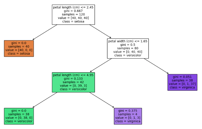
# produce classification report
y_pred = clf.predict(X_test)
print(classification_report(y_test, y_pred))
precision recall f1-score support
0 1.00 1.00 1.00 10
1 1.00 0.90 0.95 10
2 0.91 1.00 0.95 10
accuracy 0.97 30
macro avg 0.97 0.97 0.97 30
weighted avg 0.97 0.97 0.97 30 Look at the simple tree structure generated. This is far easier to understand than the unrestricted Decision Tree generated earlier. In addition, the classification report indicates this simpler model performs better! This indicates that the unrestricted model did overfit on the training data.
Post-Pruning Example
In this scenario, an unrestricted tree is grown first, and then truncated according to some criteria. Here we’ll make use of cost-complexity pruning to accomplish this task. We define a cost complexity measure R_\alpha(T) for Decision Tree T, that is parameterised by \alpha \ge 0:
R_\alpha(T) = R(T) + \alpha|\tilde{T}|
R(T) is the total impurity of the leaf nodes weighted by sample, and \tilde{T} is the number of leaf nodes in T. Note that R(T) is analogous to the training error for the tree. As \alpha increases, the more we are penalised for having larger trees. Conversely, the smaller \alpha is, the more the tree is permitted to grow without increasing the cost complexity.
The aim here is to find a sub tree of T that minimises R_\alpha(T). To achieve this, the procedure we will follow is:
- Train a Decision Tree without restrictions on the data.
- Determine the set of effective alpha parameters \alpha = \alpha_{eff} for each branch in T. A branch T_t is an interior node t in T, plus all its child nodes. The \alpha_{eff} is the value of alpha where the cost complexity of each interior node, on its own, is equal to that of its branch: R_{\alpha_{eff}}(T_t) = R_{\alpha_{eff}}(t).
- Remove branches when their \alpha_{eff} value is less than or equal to a specified threshold. Use a hyperparameter tuning technique to determine the optimal \alpha threshold value for our problem.
Let’s proceed to execute our procedure:
# step 1: fit a decision tree classifier
clf = DecisionTreeClassifier(random_state=42)
clf.fit(X_train,y_train)

# step 2: extract the set of cost complexity parameter alphas
ccp_alphas = clf.cost_complexity_pruning_path(X_train,y_train)['ccp_alphas']

# view the complete list of effective alphas
ccp_alphas.tolist()
[0.0, 0.00625, 0.00811403508771929, 0.03392857142857145, 0.2706766917293233, 0.3333333333333334]
After completing steps 1 & 2, we have a complete set of \alpha_{eff} values for this problem. Now let’s make use of GridSearchCV to finish step 3:
# setup parameter space
parameters = {'ccp_alpha':ccp_alphas.tolist()}

# create an instance of the grid search object
gsearch = GridSearchCV(DecisionTreeClassifier(random_state=42), parameters, cv=10)

# step 3: conduct grid search over the parameter space
gsearch.fit(X_train,y_train)
Now we can view the optimal \alpha_{eff} value determined by our procedure:
# show best parameter configuration found for classifier
gsearch.best_params_
{'ccp_alpha': 0.00625} Like before, let’s visualise the tree structure and produce a report on the test set:
# extract best classifier
clf = gsearch.best_estimator_

# visualise the decision tree
fig = plt.figure(figsize=(16,8))
_ = plot_tree(clf,
              feature_names=feature_names,
              filled=True,
              class_names=class_names,
              fontsize=10)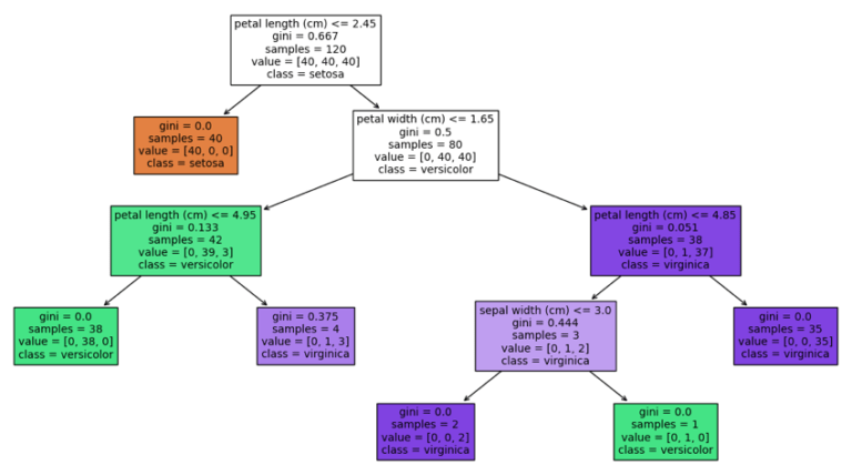
# produce classification report
y_pred = clf.predict(X_test)
print(classification_report(y_test, y_pred))
precision recall f1-score support
0 1.00 1.00 1.00 10
1 1.00 0.90 0.95 10
2 0.91 1.00 0.95 10
accuracy 0.97 30
macro avg 0.97 0.97 0.97 30
weighted avg 0.97 0.97 0.97 30 We can see that in this case, the performance results of our Post-Pruning procedure are identical to those we obtained with Pre-Pruning. However, the tree produced with Post-Pruning is more complex than the one we obtained with Pre-Pruning. Therefore, is terms of explainability, the Pre-Pruning model would be the optimal choice.
Note that in general this will not be the case. You will need to investigate which approach is best for your particular project.
Final Remarks
In this article you have learned:
- That Decision Trees tend to overfit on the training data, if their growth is not restricted in some way.
- Pruning Decision Trees involves techniques designed to combat overfitting. In effect, this is a form of regularisation.
- There are 2 different types of Pruning: Pre-Pruning and Post-Pruning.
- How to implement Pre-Pruning and Post-Pruning in Python.
I hope you enjoyed this article, and gained some value from it. If you have any questions or comments regarding this content, please write them below!
Related Posts
Hi I'm Michael Attard, a Data Scientist with a background in Astrophysics. I enjoy helping others on their journey to learn more about machine learning, and how it can be applied in industry.