Yes, Decision Trees handle categorical features naturally. Often these features are treated by first one-hot-encoding (OHE) in a preprocessing step. However, it is straightforward to extend the CART algorithm to make use of categorical features without such preprocessing. In this post, I will implement classification and regression Decision Trees capable of dealing directly with categorical features in the data.
Table of Contents
How Can Decision Trees Handle Categorical Features
In an earlier article, I covered in depth the CART algorithm, and how to implement this in Python. For that discussion, it was implicitly assumed that the data used for training, and generating predictions, comprise entirely numerical features. In a production environment this will generally not be the case: a dataset can include categorical features as well. One way to handle categorical values is to add a preprocessing step to treat for them in our machine learning pipeline. This will typically involve one-hot-encoding, to convert the string values into numerical ones. In fact, many machine learning algorithms will require such a step to be added for them to work at all.
The CART algorithm makes it possible to handle categorical features within the Decision Tree itself. We can therefore skip the additional step during preprocessing. Some modifications will be required to the algorithm, however. Below I will outline one possible approach to grow a Decision Tree, and produce predictions from a trained model, on data that include categorical features. These steps will be identical to those covered in my article on Decision Trees, with the required modifications put in bold:
Train a Decision Tree
- Select a metric upon which the decision rules will be based.
- Work out a schema for the data, that indicates whether a given feature is numeric or categorical.
- Start at the root node with all the training data.
- Choose one feature, and threshold value, by which the training data will be split that minimises our metric. For categorical features, this split will be done by selecting all samples that are equal/not-equal to the threshold value. Record the feature – threshold value pair.
- Partition the data according to the chosen feature and threshold. For categorical features, the partitioning will be done by selecting all samples that are equal/not-equal to the threshold value. Repeat steps 4 and 5 for each subset of the data.
- Stop partitioning when: i) all samples in the given node have the same label value \bold{y}, ii) a specified model limit is reached (e.g. maximum tree depth, etc.). In the terminal partitions, compute the leaf node values, and record these.
Predictions from a Trained Decision Tree
- Pass the input predictor data through the tree, starting at the root node.
- Move to either the left or right child node. The choice of moving right or left depends on how these data satisfy the decision rules (which are based on the feature – threshold pairs stored in step 4 of the training procedure). If a feature in the input is categorical, we will move left if the value is equal to the threshold, and right otherwise.
- Navigate through the tree, in the manner described by point 2, until a leaf node is reached. The stored leaf node value can then be provided as the prediction.
Modify Python Decision Tree Classes
Let’s now modify the Python code, implemented in my previous article on Decision Trees, to support categorical features. Note the complete code is available on my GitHub. In that previous article, 4 classes were defined to do the job:
- Node : this class controls the behaviour of a single node in the tree.
- DecisionTree : an abstract base class that encapsulates all the common functionality between classification and regression Decision Trees.
- DecisionTreeClassifier : a child class of DecisionTree, that encapsulates all functionality unique to classification.
- DecisionTreeRegressor : another child class of DecisionTree, that encapsulates all functionality unique to regression.
Only the DecisionTree class will require modifications. The Node, DecisionTreeClassifier, and DecisionTreeRegressor classes can be left as-is. Let’s see how the initialiser of DecisionTree will be changed:
class DecisionTree(ABC):
    """
    Base class to encompass the CART algorithm
    """

    def __init__(self, max_depth: int=None, min_samples_split: int=2) -> None:
        """
        Initializer

        Inputs:
            max_depth         -> maximum depth the tree can grow
            min_samples_split -> minimum number of samples required to split a node
        """
        self.tree              = None
        self.schema            = {} # ***CHANGES HERE***
        self.max_depth         = max_depth
        self.min_samples_split = min_samples_split
A new class member, schema, has been added. This dictionary will store the schema for the input predictor features to the model.
The private __grow function, used to build the tree during training, will also need some small changes:
    def __grow(self, node: Node, D: np.array, level: int) -> None:
        """
        Private recursive function to grow the tree during training

        Inputs:
            node  -> input tree node
            D     -> sample of data at node
            level -> depth level in the tree for node
        """
        # are we in a leaf node?
        depth = (self.max_depth is None) or (self.max_depth >= (level+1))
        msamp = (self.min_samples_split <= D.shape[0])
        n_cls = np.unique(D[:,-1]).shape[0] != 1

        # not a leaf node
        if depth and msamp and n_cls:

            # initialize the function parameters
            ip_node = None
            feature = None
            split   = None
            left_D  = None
            right_D = None
            # iterate through the possible feature/split combinations
            for f in range(D.shape[1]-1):
                for s in np.unique(D[:,f]):
                    # for the current (f,s) combination, split the dataset
                    if self.schema[f] == 'numeric': # ***CHANGES HERE***
                        D_l = D[D[:,f]<=s]
                        D_r = D[D[:,f]>s]
                    else:
                        D_l = D[D[:,f]==s]
                        D_r = D[D[:,f]!=s]
                    # ensure we have non-empty arrays
                    if D_l.size and D_r.size:
                        # calculate the impurity
                        ip  = (D_l.shape[0]/D.shape[0])*self._impurity(D_l) + (D_r.shape[0]/D.shape[0])*self._impurity(D_r)
                        # now update the impurity and choice of (f,s)
                        if (ip_node is None) or (ip < ip_node):
                            ip_node = ip
                            feature = f
                            split   = s
                            left_D  = D_l
                            right_D = D_r
            # set the current node's parameters
            node.set_params(split,feature)
            # declare child nodes
            left_node  = Node()
            right_node = Node()
            node.set_children(left_node,right_node)
            # investigate child nodes
            self.__grow(node.get_left_node(),left_D,level+1)
            self.__grow(node.get_right_node(),right_D,level+1)

        # is a leaf node
        else:

            # set the node value & return
            node.leaf_value = self._leaf_value(D)
            return
Now when splitting the data, a distinction needs to be made when dealing with categorical or numeric features. This distinction was outlined in the training procedure of the previous section.
The private __traverse function, used when generating predictions, will need changes to how one navigates through the tree:
    def __traverse(self, node: Node, Xrow: np.array) -> int | float:
        """
        Private recursive function to traverse the (trained) tree

        Inputs:
            node -> current node in the tree
            Xrow -> data sample being considered
        Output:
            leaf value corresponding to Xrow
        """
        # check if we're in a leaf node?
        if node.leaf_value is None:
            # get parameters at the node
            (s,f) = node.get_params()
            # decide to go left or right? # ***CHANGES HERE***
            if ( ((Xrow[f] <= s) & (self.schema[f] == 'numeric')) |
                ((Xrow[f] == s) & (self.schema[f] == 'categorical')) ):
                return(self.__traverse(node.get_left_node(),Xrow))
            else:
                return(self.__traverse(node.get_right_node(),Xrow))
        else:
            # return the leaf value
            return(node.leaf_value)
Like with __grow, changes needed to be introduced here to account for categorical features. These changes were outlined in the prediction procedure outlined in the previous section.
The final changes needed to DecisionTree will be placed within the public train member function:
    def train(self, Xin: np.array, Yin: np.array) -> None:
        """
        Train the CART model

        Inputs:
            Xin -> input set of predictor features
            Yin -> input set of labels
        """
        # check data schema ***CHANGES HERE***
        self.schema = {}
        for f in range(Xin.shape[1]):
            try:
                _ = Xin[:,f].astype(float)
                self.schema[f] = 'numeric'
            except:
                self.schema[f] = 'categorical'
        # prepare the input data
        D = np.concatenate((Xin,Yin.reshape(-1,1)),axis=1)
        # set the root node of the tree
        self.tree = Node()
        # build the tree
        self.__grow(self.tree,D,1)
Here the schema for the input predictor features is determined first, before building the tree.
This encompasses all the changes required to support categorical features. We can now proceed to test out our implementation with classification and regression examples.
Classification Example with Categorical Features
Let’s test out the classification model, using a simulated dataset consisting of 1000 samples, 5 predictive features, and 2 distinct class labels. This dataset will be comprised of two distinct populations, that are then combined. The second population will consist of input features that have been shifted and scaled, with respect to the first.
I will make two versions of the aforementioned dataset. These two versions will differ in the way the two component populations are flagged.
The first dataset distinguishes between these two populations with a single categorical column. The entries in this column are a and b, where each letter represents a different population.
The second dataset distinguishes between these two populations with one-hot-encoding. As a result, two columns are added to make this distinction.
# create a classification datasets
X1,y1 = make_classification(n_samples=500, n_features=5, n_classes=2, random_state=42)
X2,y2 = make_classification(n_samples=500, n_features=5, n_classes=2, shift=5.0, scale=2.0, random_state=24)
# assemble dataset with categorical feature
cat1   = np.array(['a' for _ in range(X1.shape[0])],dtype='object').reshape(-1,1)
cat2   = np.array(['b' for _ in range(X1.shape[0])],dtype='object').reshape(-1,1)
X1_cat = np.append(X1, cat1, axis=1)
X2_cat = np.append(X2, cat2, axis=1)
X_cat  = np.concatenate((X1_cat, X2_cat), axis=0)
# assemble dataset with OHE feature
cat1   = np.append(np.ones((X1.shape[0],1)), np.zeros((X1.shape[0],1)), axis=1)
cat2   = np.append(np.zeros((X1.shape[0],1)), np.ones((X1.shape[0],1)), axis=1)
X1_ohe = np.append(X1, cat1, axis=1)
X2_ohe = np.append(X2, cat2, axis=1)
X_ohe  = np.concatenate((X1_ohe, X2_ohe), axis=0)
# assemble label
y = np.concatenate((y1,y2), axis=0)
Since I did not specify the weights argument in make_classification, we can conclude these data are balanced.
X_cat is the set of predictor features that include a categorical feature. On the other hand, X_ohe has the same input features, but with two OHE columns instead of the single categorical one.
Let’s plot the predictor features, to see what we have generated:
# box plot of features
plt.boxplot(np.append(X1, X2, axis=1))
plt.xlabel('features')
plt.ylabel('values')
plt.title('Distributions in Features')
plt.xticks([1, 2, 3, 4, 5, 6, 7, 8, 9, 10],
           ['x1_a', 'x2_a', 'x3_a', 'x4_a', 'x5_a', 'x1_b', 'x2_b', 'x3_b', 'x4_b', 'x5_b'])
plt.show()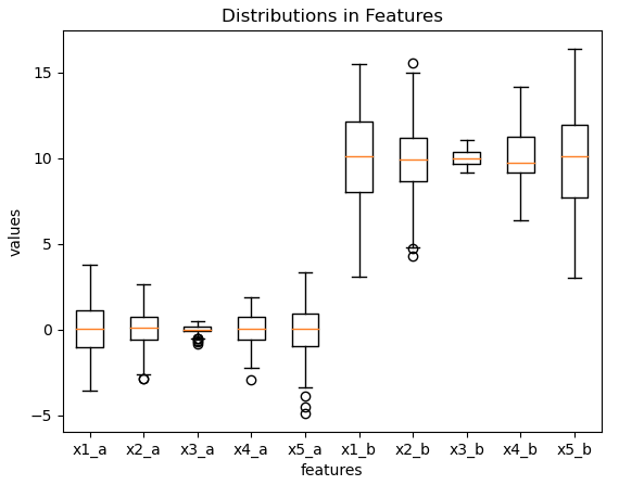
The two distinct populations of predictor features are apparent. We can visually confirm the effects of scaling and shifting the 5 b features, with respect to the a features.
Let’s view the first few rows of our data:
# view of predictor features with categorical column
X_cat[:3,:]
array([[1.3930969851746609, -0.9683444548636353, -0.38159403502172495,
-1.2583346392630976, -2.613270726882727, 'a'],
[-0.9401485204629451, 1.1906462747863413, 0.1868405676603463,
0.37796097806297374, 1.0210120505425357, 'a'],
[0.6954945017358167, 0.9278401280812372, 0.0628733980199353,
1.0610773601766177, 1.3573407167599494, 'a']], dtype=object) # view of predictor features with OHE columns
X_ohe[:3,:]array([[ 1.39309699, -0.96834445, -0.38159404, -1.25833464, -2.61327073,
1. , 0. ],
[-0.94014852, 1.19064627, 0.18684057, 0.37796098, 1.02101205,
1. , 0. ],
[ 0.6954945 , 0.92784013, 0.0628734 , 1.06107736, 1.35734072,
1. , 0. ]]) It is clear that the two sets of predictor features are the same, except for the final column in X_cat and the last two columns in X_ohe.
We can now proceed with a train-test split of these data, where 20% of the samples will be held-out for testing:
# do train/test split
X_cat_train, X_cat_test, X_ohe_train, X_ohe_test, y_train, y_test = train_test_split(X_cat,
                                                                                     X_ohe,
                                                                                     y,
                                                                                     test_size=0.2,
                                                                                     random_state=42)
The next steps will involve declaring an instance of our custom classifier, and training it on the categorical data. Once this is done, we can print out the schema to verify our expectations:
# train an instance of the custom decision tree classifier
clf = DecisionTreeClassifier(max_depth=5)
clf.train(X_cat_train,y_train)

# view the learned schema
clf.schema
{0: 'numeric',
1: 'numeric',
2: 'numeric',
3: 'numeric',
4: 'numeric',
5: 'categorical'} Training proceeded without issue, and the resulting schema correctly indicates the first 5 features as being numeric. Only the 6th feature is categorical.
Now let’s generate predictions on the test set with our trained custom classifier. We can then measure the performance by comparing these predictions with the test set labels:
# generate predictions
yp = clf.predict(X_cat_test)

# evaluate model performance
print("accuracy: %.2f" % accuracy_score(y_test,yp))
print("precision: %.2f" % precision_score(y_test,yp))
print("recall: %.2f" % recall_score(y_test,yp))
accuracy: 0.88 precision: 0.83 recall: 0.95
These results look good. Let’s compare these values with the performance of the scikit-learn Decision Tree classifier on the OHE data:
# compare with OHE data & scikit-learn classifier
from sklearn.tree import DecisionTreeClassifier
clf = DecisionTreeClassifier(max_depth=5)
clf.fit(X_ohe_train,y_train)

# generate predictions
yp = clf.predict(X_ohe_test)

# evaluate model performance
print("accuracy: %.2f" % accuracy_score(y_test,yp))
print("precision: %.2f" % precision_score(y_test,yp))
print("recall: %.2f" % recall_score(y_test,yp))
accuracy: 0.86 precision: 0.84 recall: 0.92
The results between the two models are approximately consistent. This indicates that our custom implementation, with a categorical feature, works as hoped. Therefore it is possible to build Decision Tree classifiers that can handle categorical features, without the need to carry out a preprocessing step (like OHE).
Regression Example with Categorical Features
Similarly to what was done with the classification example, we can now test our custom Decision Tree regressor. Let’s start by creating a synthetic dataset with scikit-learn’s make_regression function. Two calls to this function will be made, to generate a dataset consisting of 1000 samples, 5 predictive features, and 1 target. This dataset will be comprised of two distinct populations, that are then combined. The second population will have a y-intercept for the target that is offset by 200.0, with respect to the first population.
I will make two versions of the aforementioned dataset. These two versions will differ in the way the two component populations are flagged.
The first dataset will distinguish between these two populations with a single categorical column. The entries in this column will be a and b.
The second dataset will distinguish between these two populations with one-hot-encoding. As a result, two columns will be added here.
# create a classification datasets
X1,y1 = make_regression(n_samples=500, n_features=5, n_targets=1, noise=0.1, random_state=42)
X2,y2 = make_regression(n_samples=500, n_features=5, n_targets=1, bias=200.0, noise=0.2, random_state=24)
# assemble dataset with categorical feature
cat1   = np.array(['a' for _ in range(X1.shape[0])],dtype='object').reshape(-1,1)
cat2   = np.array(['b' for _ in range(X1.shape[0])],dtype='object').reshape(-1,1)
X1_cat = np.append(X1, cat1, axis=1)
X2_cat = np.append(X2, cat2, axis=1)
X_cat  = np.concatenate((X1_cat, X2_cat), axis=0)
# assemble dataset with OHE feature
cat1   = np.append(np.ones((X1.shape[0],1)), np.zeros((X1.shape[0],1)), axis=1)
cat2   = np.append(np.zeros((X1.shape[0],1)), np.ones((X1.shape[0],1)), axis=1)
X1_ohe = np.append(X1, cat1, axis=1)
X2_ohe = np.append(X2, cat2, axis=1)
X_ohe  = np.concatenate((X1_ohe, X2_ohe), axis=0)
# assemble label
y = np.concatenate((y1,y2), axis=0)
Like classification example, X_cat is the set of predictor features that include a categorical feature. On the other hand, X_ohe has the same input features, but with two OHE columns instead of the single categorical one.
Let’s plot the predictor features, and the distributions in the target we have generated:
# box plot of features
plt.boxplot(np.append(X1, X2, axis=1))
plt.xlabel('features')
plt.ylabel('values')
plt.title('Distributions in Features')
plt.xticks([1, 2, 3, 4, 5, 6, 7, 8, 9, 10],
           ['x1_a', 'x2_a', 'x3_a', 'x4_a', 'x5_a', 'x1_b', 'x2_b', 'x3_b', 'x4_b', 'x5_b'])
plt.show()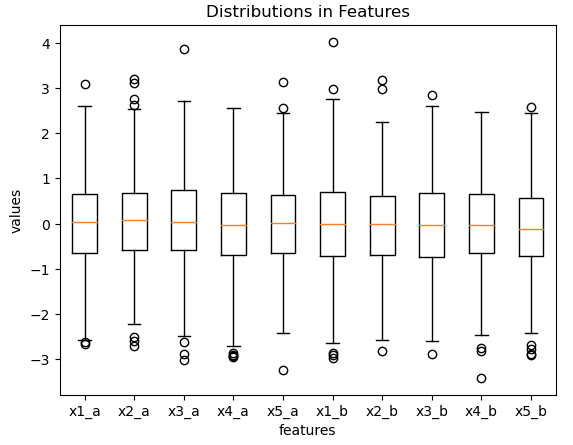
# histogram of target
plt.hist(y,bins=50,label='a+b')
plt.hist(y1,bins=50,label='a')
plt.hist(y2,bins=50,label='b')
plt.xlabel('y target')
plt.ylabel('frequency')
plt.title('Distributions in y Target')
plt.legend()
plt.show()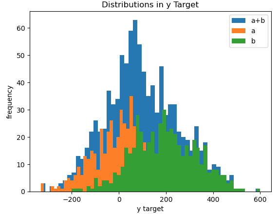
This time we do not see much variation in the input predictor features, as we would expect. However, the differences between the two populations are apparent when we look at the target. The histogram above illustrates the shift introduced between population a (in orange) and population b (in green). Blue indicates the distribution of the net combined population a+b.
Let’s view the first few rows of our predictor features:
# view of predictor features with categorical column
X_cat[:3,:]
array([[0.5609194479412387, -0.3700110298821277, -0.29548031802916036,
-0.25879606266710237, 1.598647170504717, 'a'],
[-1.0243876413342898, -0.926930471578083, -0.2525681513931603,
-0.05952535606180008, -3.2412673400690726, 'a'],
[-2.650969808393012, 0.10643022769189683, 1.0915068519224618,
-0.2549772174208553, 1.5039929885826886, 'a']], dtype=object) # view of predictor features with OHE columns
X_ohe[:3,:]array([[ 0.56091945, -0.37001103, -0.29548032, -0.25879606, 1.59864717,
1. , 0. ],
[-1.02438764, -0.92693047, -0.25256815, -0.05952536, -3.24126734,
1. , 0. ],
[-2.65096981, 0.10643023, 1.09150685, -0.25497722, 1.50399299,
1. , 0. ]]) We can see that the two sets of predictor features are the same, except for the final column in X_cat and the last two columns in X_ohe.
Let’s now do a train-test split of these data, with 20% being held-out for testing. Afterwards, we can train an instance of our custom Decision Tree regressor:
# do train/test split
X_cat_train, X_cat_test, X_ohe_train, X_ohe_test, y_train, y_test = train_test_split(X_cat,
                                                                                     X_ohe,
                                                                                     y,
                                                                                     test_size=0.2,
                                                                                     random_state=42)

# train an instance of the custom decision tree regressor
rgr = DecisionTreeRegressor(max_depth=5)
rgr.train(X_cat_train,y_train)
With training done, we can print out the schema to confirm the feature types have been detected correctly:
# view the learned schema
rgr.schema
{0: 'numeric',
1: 'numeric',
2: 'numeric',
3: 'numeric',
4: 'numeric',
5: 'categorical'} The schema correctly indicates the first 5 features as being numeric. Only the 6th feature is categorical.
Now let’s generate predictions on the test set with our trained custom regressor. We can then record the mean absolute error and mean squared error by comparing these predictions with the test set labels:
# generate predictions
yp = rgr.predict(X_cat_test)

# evaluate model performance
print("mae: %.2f" % mean_absolute_error(y_test,yp))
print("mse: %.2f" % mean_squared_error(y_test,yp))
mae: 66.58 mse: 7157.99
These results look good. Let’s compare these values with the performance of the scikit-learn Decision Tree regressor on the OHE data:
# compare with OHE data & scikit-learn regressor
from sklearn.tree import DecisionTreeRegressor
rgr = DecisionTreeRegressor(max_depth=5)
rgr.fit(X_ohe_train,y_train)

# generate predictions
yp = rgr.predict(X_ohe_test)

# evaluate model performance
print("mae: %.2f" % mean_absolute_error(y_test,yp))
print("mse: %.2f" % mean_squared_error(y_test,yp))
mae: 65.18 mse: 6864.23
The results between the two models are approximately consistent, indicating that our custom implementation with a categorical feature works as hoped. This shows that it is possible to build a Decision Tree regressor that can handle categorical features, without the need to carry out a preprocessing step (like OHE).
Final Remarks
In this article you have learned:
- That Decision Trees can handle categorical features in the data.
- One possible approach to how CART Decision Trees can be modified to handle categorical features.
- An actual Python implementation of Decision Trees that can support categorical features.
Please feel free to visit my GitHub page, where I have the complete Python code presented here in a single jupyter notebook. Download the notebook, and play around with the implementation. If you have any questions or comments, please leave them below!
Related Posts
Hi I'm Michael Attard, a Data Scientist with a background in Astrophysics. I enjoy helping others on their journey to learn more about machine learning, and how it can be applied in industry.