Introduction

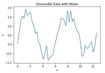
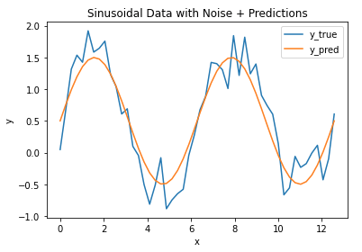
In this post we’ll cover the Mean Squared Error (MSE), arguably one of the most popular error metrics for regression analysis. The MSE is expressed as:

MSE = \frac{1}{N}\sum_i^N(\hat{y}_i-y_i)^2    (1)

where \hat{y}_i are the model output and y_i are the true values. The summation is performed over N individual data points available in our sample.

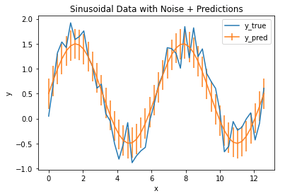
The advantage of the MSE is that it is easily differentiated, making it ideal for optimisation analysis. In addition, we can interpret the MSE in terms of the bias and variance in the model. We can see this is the case by expressing (1) in terms of expected values, and then expanding the squared difference:

MSE = E[(\hat{y}-y)^2]

   = E[\hat{y}^2 + y^2 – 2\hat{y}y]

We can now add positive and negative E(\hat{y})^2 terms, and make use of our definitions of bias and variance:

   = E(\hat{y}^2) – E(\hat{y})^2 + E(\hat{y})^2 + y^2 – 2yE(\hat{y})

   = Var(\hat{y}) + E(\hat{y})^2 – 2yE(\hat{y}) + y^2

   = Var(\hat{y}) + E[\hat{y} – y]^2

   = Var(\hat{y}) + Bias^2(\hat{y})

One complication of using the MSE is the fact that this error metric is expressed in termed of squared units. To express the error in terms of the units of y and \hat{y}, we can compute the Root Mean Squared Error (RMSE):

RMSE = \sqrt{MSE}    (2)

In addition, the MSE tends to be much more sensitive the outliers when compared to other metrics, such as the mean absolute error or making use of the median.

Python Coding Example

Here I will make use of the same example used when demonstrating the mean absolute error. First let’s import the required packages:

## imports ##
import numpy as np
from sklearn.metrics import mean_squared_error
import matplotlib.pyplot as plt

Notice that scikit-learn provides a function for computing the MSE. Like before, let’s create the toy data set and plot the results:

## define two arrays: x & y ##
x_true = np.linspace(0,4*np.pi,50)
y_true = np.sin(x_true) + np.random.rand(x_true.shape[0])

## plot the data ##
plt.plot(x_true,y_true)
plt.title('Sinusoidal Data with Noise')
plt.xlabel('x')
plt.ylabel('y')
plt.show()
mean squared error

 Let’s now assume we have a model that is fitted to these data. We can make a plot of this model together with the raw data:

## plot the data & predictions ##
plt.plot(x_true,y_true)
plt.plot(x_true,y_pred)
plt.title('Sinusoidal Data with Noise + Predictions')
plt.xlabel('x')
plt.ylabel('y')
plt.legend(['y_true','y_pred'])
plt.show()
mean squared error

We can see that the model follows the general pattern in the data, however there are differences between the two. We can measure the magnitude of these differences  by computing the MSE (and RMSE):

## compute the mse ##
mse = mean_squared_error(y_true,y_pred)
print("The mean sqaured error is: {:.2f}".format(mse))
print("The root mean squared error is: {:.2f}".format(np.sqrt(mse)))

The mean sqaured error is: 0.09

The root mean squared error is: 0.30

Remember that the RMSE is in the same units as the data themselves. We can directly compare the RMSE with the MAE computed in an earlier post. The RMSE here (0.30) is slightly larger than the MAE (0.27), which is expected as the squared error is more sensitive to large differences between the model and data. 

Finally, we can plot the RMSE as vertical error bars on top of our model output:

## plot the data & predictions with the rmse ##
plt.plot(x_true,y_true)
plt.errorbar(x_true,y_pred,np.sqrt(mse))
plt.title('Sinusoidal Data with Noise + Predictions')
plt.xlabel('x')
plt.ylabel('y')
plt.legend(['y_true','y_pred'])
plt.show()
mean squared error

The error bars define the region of uncertainty for our model, and we can see that it covers the bulk of the fluctuations in the data.  As such, we can conclude that the MSE/RMSE does a good job at quantifying the error in our model output.

Related Posts

0 0 votes
Article Rating
Subscribe
Notify of
guest

1 Comment
Oldest
Newest Most Voted
Inline Feedbacks
View all comments
trackback

[…] The Median Absolute Error is a metric that can be used to quantify a regression models performance. This measure is slightly more difficult to interpret for a non-technical audience. However, the main benefit of using this quantity is its strong resilience to outliers. This is in contrast to other metrics previous discussed, such as the Mean Absolute Error or Mean Squared Error. […]

1
0
Would love your thoughts, please comment.x
()
x
Newsletter Signup