What is the Median Absolute Error?
The Median Absolute Error is a metric that can be used to quantify a regression models performance. This measure is slightly more difficult to interpret for a non-technical audience. However, the main benefit of using this quantity is its strong resilience to outliers. This is in contrast to other metrics previous discussed, such as the Mean Absolute Error or Mean Squared Error.
As its namesake would suggest, the Median Absolute Error is the median difference between the observations (true values) and model output (predictions). The sign of these differences is ignored so that cancellations between positive and negative values do not occur. If we didn’t ignore the sign, the error calculated would likely be far lower than the true difference between model and data.
Mathematically, the Median Absolute Error is expressed as:
\text{Median Absolute Error} = \text{median}|y_{i,pred}-y_{i,true}|
where y_{i,pred} are the predicted values, and y_{i,true} are the observations, for all i samples.
Let’s demonstrate the properties of the Median Absolute Error through a worked example in Python!
Python Coding Example
We can begin by importing the necessary packages required:
# imports
import numpy as np
from sklearn.metrics import median_absolute_error, mean_absolute_error, mean_squared_error
import matplotlib.pyplot as plt
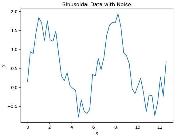
The next step will involve creating a toy dataset. In this case, I’ll generate these data using a sine curve with noise added:
# define two arrays: x & y
x_true = np.linspace(0,4*np.pi,50)
y_true = np.sin(x_true) + np.random.rand(x_true.shape[0])
Let’s plot these data to see what we’ve got:
# plot the data
plt.plot(x_true,y_true)
plt.title('Sinusoidal Data with Noise')
plt.xlabel('x')
plt.ylabel('y')
plt.show()
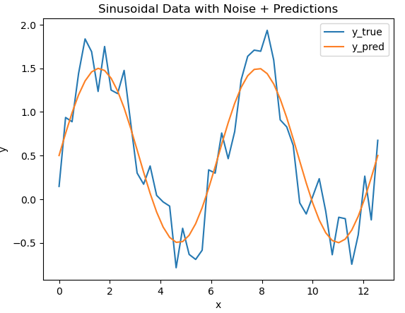
We can assume a model has been built to predict y for every x in our dataset. Let’s superimpose the predictions, from this hypothetical model, onto our data:
# plot the data & predictions
plt.plot(x_true,y_true)
plt.plot(x_true,y_pred)
plt.title('Sinusoidal Data with Noise + Predictions')
plt.xlabel('x')
plt.ylabel('y')
plt.legend(['y_true','y_pred'])
plt.show()
It is evident that the model follows the general pattern in the data. However, differences are present between the two. How can we quantify the extent of these differences? Let’s address this by calculating the error using 3 different approaches. These will include the mean_absolute_error, mean_squared_error, and median_absolute_error functions available from scikit-learn:
def print_error_metrics(y_true: np.array, y_pred: np.array) -> None:
    """
    Function to compute the mean absolute error, mean squared error, and median absolute error and print to screen

    Inputs:
        y_true -> array containing actual dependant variable
        y_pred -> array containing model predictions
    """
    mee = median_absolute_error(y_true,y_pred)
    mae = mean_absolute_error(y_true,y_pred)
    mse = mean_squared_error(y_true,y_pred)
    print("The median absolute error is: {:.2f}".format(mee))
    print("The mean absolute error is: {:.2f}".format(mae))
    print("The root mean squared error is: {:.2f}".format(np.sqrt(mse)))

# compute error metrics
print_error_metrics(y_true, y_pred)
The median absolute error is: 0.24 The mean absolute error is: 0.26 The root mean squared error is: 0.29
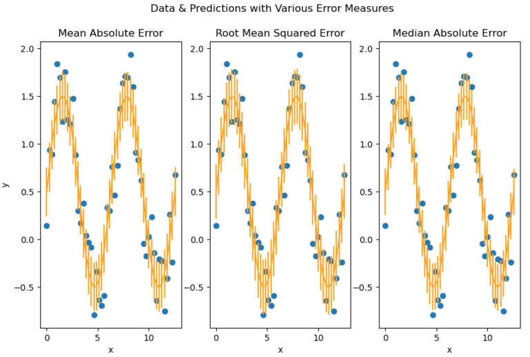
It is apparent that all of the error metrics roughly agree on the amount of discrepancy between our model and data. Let’s plot out these results to visualise what we have:
def plot_error_metrics(x_true: np.array,
                       y_true: np.array,
                       y_pred: np.array,
                       mae: float,
                       mse: float,
                       mee: float) -> None:
    """
    Function to plot data, model predictions, and error metrics in a tiled figure

    Inputs:
        x_true -> array containing predictor variable
        y_true -> array containing actual dependant variable
        y_pred -> array containing model predictions
        mae -> mean absolute error
        mse -> mean squared error
        mee -> median absolute error
    """
    fig, (ax0, ax1, ax2) = plt.subplots(nrows=1, ncols=3, sharex=True,
                                    figsize=(10, 6))

    ax0.set_title('Mean Absolute Error')
    ax0.scatter(x_true,y_true)
    ax0.errorbar(x_true, y_pred, yerr=mae, color='orange')
    ax0.set_xlabel('x')
    ax0.set_ylabel('y')

    ax1.set_title('Root Mean Squared Error')
    ax1.scatter(x_true,y_true)
    ax1.errorbar(x_true, y_pred, yerr=np.sqrt(mse), color='orange')
    ax1.set_xlabel('x')

    ax2.set_title('Median Absolute Error')
    ax2.scatter(x_true,y_true)
    ax2.errorbar(x_true, y_pred, yerr=mee, color='orange')
    ax2.set_xlabel('x')

    fig.suptitle('Data & Predictions with Various Error Measures')
    plt.show()

# plot results
plot_error_metrics(x_true, y_true, y_pred, mae, mse, mee)
Vertical bars represent the magnitude of the error calculated. We can see that the bulk of the variation seen in these data are covered by the error bars. Also, no significant differences are apparent between the different error metrics used.
Now let’s add some outliers, and check how these results change. To accomplish this, I’ll artificially introduce 3 outliers into the dependant variable y_{true}:
# add 3 outliers to the data
idx = np.random.choice([x for x in range(y_true.shape[0])],size=3)
y_true[idx] = y_true[idx]*10
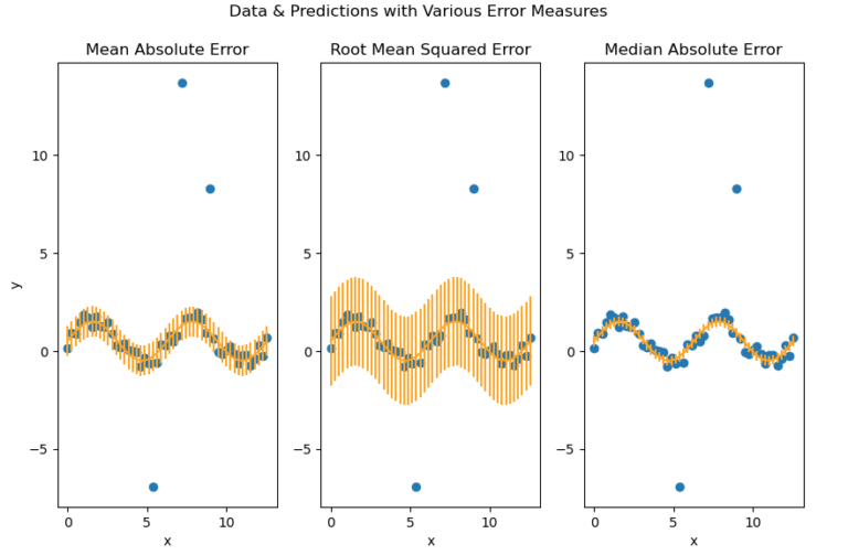
Next we can recalculate our error metrics and plot them in the same way as done before:
# compute error metrics
print_error_metrics(y_true, y_pred)
The median absolute error is: 0.25 The mean absolute error is: 0.77 The root mean squared error is: 2.26
# plot results
plot_error_metrics(x_true, y_true, y_pred, mae, mse, mee)
It is now quite apparent that our error metrics yield different results! The Mean Absolue Error shows some increase due to the presence of outliers, while the Mean Squared Error has dramatically increased. The latter error measure is particularly sensitive to the presence of outliers. Note that the 3 outliers are clearly visible in the scatter plot.
In contrast, the Median Absolute Error has not significantly changed at all. This metric is highly robust to outliers, and will yield an error measure that is representative of the vast majority of the data.
