Yes, Decision Trees handle missing values naturally. It is straightforward to extend the CART algorithm to support the handling of missing values. However, attention needs to be made regarding how the algorithm is implemented in code. In this post, I will implement classification and regression Decision Trees capable of dealing with missing values in the data.
Table of Contents
How Can Decision Trees Handle Missing Values
In an earlier article, I covered in depth the CART algorithm, and how to implement this in Python. For that discussion, it was implicitly assumed that the data used for training, and generating predictions, have no missing values. Real-life data, obtained in a production setting, will typically not meet this assumption. One way to handle missing values is to add a preprocessing step to treat for them in our machine learning pipeline. In fact, many machine learning algorithms will require such a step to be added in order to prevent software failures during operations.
The CART algorithm makes it possible to handle missing values within the Decision Tree itself. We can therefore skip the additional step during preprocessing. Some modifications will be required to the algorithm, however. Below I will outline one possible approach to grow a Decision Tree, and produce predictions from a trained model, on data with missing values. These steps will be identical to those covered in my article on Decision Trees, with the required modifications put in bold:
Train a Decision Tree
- Decide how samples with missing values will be passed to the child nodes. This decision can be treated as a hyperparameter.
- Select a metric upon which the decision rules will be based.
- Start at the root node with all the training data.
- Choose one feature, and threshold value, by which the training data will be split that minimises our metric. Check to ensure the threshold value is a defined number (not a NaN or None). Record the feature – threshold value pair.
- Partition the data according to the chosen feature and threshold, then repeat steps 4 and 5 for each subset of the data. If a sample upon which we are applying the decision rule has a missing value, move the sample according to the decision made in step 1 above.
- Stop partitioning when: i) all samples in the given node have the same non-missing label value \bold{y}, ii) a specified model limit is reached (e.g. maximum tree depth, etc.). In the terminal partitions, compute the leaf node values while omitting any missing values in the label, and record these.
Predictions from a Trained Decision Tree
- Pass the input predictor data through the tree, starting at the root node.
- Move to either the left or right child node. The choice of moving right or left depends on how these data satisfy the decision rules (which are based on the feature – threshold pairs stored in step 3 of the training procedure). If our input is a missing value, this move will be based on our decision from point 1 of the training procedure.
- Navigate through the tree, in the manner described by point 2, until a leaf node is reached. The stored leaf node value can then be provided as the prediction.
Modify Python Decision Tree Classes
Let’s now modify the Python code, implemented in my previous article on Decision Trees, to support missing values. Note the complete code is available on my GitHub. In that previous article, 4 classes were defined to do the job:
- Node : this class controls the behaviour of a single node in the tree.
- DecisionTree : an abstract base class that encapsulates all the common functionality between classification and regression Decision Trees.
- DecisionTreeClassifier : a child class of DecisionTree, that encapsulates all functionality unique to classification.
- DecisionTreeRegressor : another child class of DecisionTree, that encapsulates all functionality unique to regression.
The Node class will be unchanged, and so we can move along to the implementation of DecisionTree. A new boolean hyperparameter will be introduced: nans_go_right. This will be used to decide how input samples with missing values will be moved within the tree:
class DecisionTree(ABC):
    """
    Base class to encompass the CART algorithm
    """

    def __init__(self, max_depth: int=None, min_samples_split: int=2, nans_go_right=True) -> None:
        """
        Initializer

        Inputs:
            max_depth         -> maximum depth the tree can grow
            min_samples_split -> minimum number of samples required to split a node
            nans_go_right     -> boolean to determine where NaN values in predictors are allocated
        """
        self.tree              = None
        self.max_depth         = max_depth
        self.min_samples_split = min_samples_split
        self.nans_go_right     = nans_go_right
Private functions will also be added to control how samples flow through the tree. These will make use of nans_go_right:
    def __split_right(self, feature_col: np.array, split_point: float) -> np.array:
        """
        Private function to determine which elements in the feature column go to the child right node

        Inputs:
            feature_col -> feature column to analyse
            split_point -> split point for the feature column
        Outputs:
            numpy array of boolean values
        """
        return (feature_col > split_point) | (np.isnan(feature_col) & self.nans_go_right)

    def __split_left(self, feature_col: np.array, split_point: float) -> np.array:
        """
        Private function to determine which elements in the feature column go to the child left node

        Inputs:
            feature_col -> feature column to analyse
            split_point -> split point for the feature column
        Outputs:
            numpy array of boolean values
        """
        return (feature_col <= split_point) | (np.isnan(feature_col) & (not self.nans_go_right))
The private recursive function __grow, that is used to grow the Decision Tree during training, will also have some modifications. These mainly center around ensuring NaN’s don’t leak into our calculations. We will also make use of the functions defined above, __split_right and __split_left, to determine how the data are split at every non-leaf node:
    def __grow(self, node: Node, D: np.array, level: int) -> None:
        """
        Private recursive function to grow the tree during training

        Inputs:
            node  -> input tree node
            D     -> sample of data at node
            level -> depth level in the tree for node
        """
        # are we in a leaf node?
        depth = (self.max_depth is None) or (self.max_depth >= (level+1))
        msamp = (self.min_samples_split <= D.shape[0])
        cls   = D[:,-1]
        n_cls = np.unique(cls[~np.isnan(cls)]).shape[0] != 1

        # not a leaf node
        if depth and msamp and n_cls:

            # initialize the function parameters
            ip_node = None
            feature = None
            split   = None
            left_D  = None
            right_D = None
            # iterate through the possible feature/split combinations
            for f in range(D.shape[1]-1):
                f_values = D[:,f]
                for s in np.unique(f_values[~np.isnan(f_values)]):
                    # for the current (f,s) combination, split the dataset
                    D_l = D[self.__split_left(D[:,f],s)]
                    D_r = D[self.__split_right(D[:,f],s)]
                    # ensure we have non-empty arrays
                    if D_l.size and D_r.size:
                        # calculate the impurity
                        ip  = (D_l.shape[0]/D.shape[0])*self._impurity(D_l) + (D_r.shape[0]/D.shape[0])*self._impurity(D_r)
                        # now update the impurity and choice of (f,s)
                        if (ip_node is None) or (ip < ip_node):
                            ip_node = ip
                            feature = f
                            split   = s
                            left_D  = D_l
                            right_D = D_r
            # set the current node's parameters
            node.set_params(split,feature)
            # declare child nodes
            left_node  = Node()
            right_node = Node()
            node.set_children(left_node,right_node)
            # investigate child nodes
            self.__grow(node.get_left_node(),left_D,level+1)
            self.__grow(node.get_right_node(),right_D,level+1)

        # is a leaf node
        else:

            # set the node value & return
            node.leaf_value = self._leaf_value(D)
            return
The private recursive function __traverse will also be adapted to make use of __split_left:
    def __traverse(self, node: Node, Xrow: np.array) -> int | float:
        """
        Private recursive function to traverse the (trained) tree

        Inputs:
            node -> current node in the tree
            Xrow -> data sample being considered
        Output:
            leaf value corresponding to Xrow
        """
        # check if we're in a leaf node?
        if node.leaf_value is None:
            # get parameters at the node
            (s,f) = node.get_params()
            # decide to go left or right?
            if (self.__split_left(Xrow[f],s)):
                return(self.__traverse(node.get_left_node(),Xrow))
            else:
                # note nan's in Xrow will go right
                return(self.__traverse(node.get_right_node(),Xrow))
        else:
            # return the leaf value
            return(node.leaf_value)
I included some minor changes to the train and predict functions, that aim at converting ‘None’ values to numpy ‘NaN’:
    def train(self, Xin: np.array, Yin: np.array) -> None:
        """
        Train the CART model

        Inputs:
            Xin -> input set of predictor features
            Yin -> input set of labels
        """
        # prepare the input data
        D            = np.concatenate((Xin,Yin.reshape(-1,1)),axis=1)
        D[D == None] = np.nan
        D            = D.astype('float64')
        # set the root node of the tree
        self.tree = Node()
        # build the tree
        self.__grow(self.tree,D,1)

    def predict(self, Xin: np.array) -> np.array:
        """
        Make predictions from the trained CART model

        Input:
            Xin -> input set of predictor features
        Output:
            array of prediction values
        """
        # prepare the input data
        Xin[Xin == None] = np.nan
        Xin              = Xin.astype('float64')
        # iterate through the rows of Xin
        p = []
        for r in range(Xin.shape[0]):
            p.append(self.__traverse(self.tree,Xin[r,:]))
        # return predictions
        return(np.array(p).flatten())
Let’s now proceed to DecisionTreeClassifier. The changes to this class consist of:
- adding the new hyperparameter, nans_go_right
- ensuring NaN values do not leak into impurity or leaf node value calculations
class DecisionTreeClassifier(DecisionTree):
    """
    Decision Tree Classifier
    """

    def __init__(self, max_depth: int=None, min_samples_split: int=2, nans_go_right=True, loss: str='gini') -> None:
        """
        Initializer

        Inputs:
            max_depth         -> maximum depth the tree can grow
            min_samples_split -> minimum number of samples required to split a node
            nans_go_right     -> boolean to determine where NaN values in predictors are allocated
            loss              -> loss function to use during training
        """
        DecisionTree.__init__(self,max_depth,min_samples_split,nans_go_right)
        self.loss = loss

    def __gini(self, D: np.array) -> float:
        """
        Private function to define the gini impurity

        Input:
            D -> data to compute the gini impurity over
        Output:
            Gini impurity for D
        """
        # initialize the output
        G = 0
        # iterate through the unique classes
        cls = D[:,-1]
        for c in np.unique(cls[~np.isnan(cls)]):
            # compute p for the current c
            p = D[D[:,-1]==c].shape[0]/D.shape[0]
            # compute term for the current c
            G += p*(1-p)
        # return gini impurity
        return(G)

    def __entropy(self, D: np.array) -> float:
        """
        Private function to define the shannon entropy

        Input:
            D -> data to compute the shannon entropy over
        Output:
            Shannon entropy for D
        """
        # initialize the output
        H = 0
        # iterate through the unique classes
        cls = D[:,-1]
        for c in np.unique(cls[~np.isnan(cls)]):
            # compute p for the current c
            p = D[D[:,-1]==c].shape[0]/D.shape[0]
            # compute term for the current c
            H -= p*np.log2(p)
        # return entropy
        return(H)

    def _impurity(self, D: np.array) -> float:
        """
        Protected function to define the impurity

        Input:
            D -> data to compute the impurity metric over
        Output:
            Impurity metric for D
        """
        # use the selected loss function to calculate the node impurity
        ip = None
        if self.loss == 'gini':
            ip = self.__gini(D)
        elif self.loss == 'entropy':
            ip = self.__entropy(D)
        # return results
        return(ip)

    def _leaf_value(self, D: np.array) -> int:
        """
        Protected function to compute the value at a leaf node

        Input:
            D -> data to compute the leaf value
        Output:
            Mode of D
        """
        return(stats.mode(D[:,-1],keepdims=False,nan_policy='omit')[0])
Similar changes are also required for the DecisionTreeRegressor class:
class DecisionTreeRegressor(DecisionTree):
    """
    Decision Tree Regressor
    """

    def __init__(self, max_depth: int=None, min_samples_split: int=2, nans_go_right=True, loss: str='mse') -> None:
        """
        Initializer

        Inputs:
            max_depth         -> maximum depth the tree can grow
            min_samples_split -> minimum number of samples required to split a node
            nans_go_right     -> boolean to determine where NaN values in predictors are allocated
            loss              -> loss function to use during training
        """
        DecisionTree.__init__(self,max_depth,min_samples_split,nans_go_right)
        self.loss = loss

    def __mse(self, D: np.array) -> float:
        """
        Private function to define the mean squared error

        Input:
            D -> data to compute the MSE over
        Output:
            Mean squared error over D
        """
        # compute the mean target for the node
        y_m = np.mean(D[:,-1],where=~np.isnan(D[:,-1]))
        # compute the mean squared error wrt the mean
        E = np.sum((D[:,-1] - y_m)**2,where=~np.isnan(D[:,-1]))/D.shape[0]
        # return mse
        return(E)

    def __mae(self, D: np.array) -> float:
        """
        Private function to define the mean absolute error

        Input:
            D -> data to compute the MAE over
        Output:
            Mean absolute error over D
        """
        # compute the mean target for the node
        y_m = np.mean(D[:,-1],where=~np.isnan(D[:,-1]))
        # compute the mean absolute error wrt the mean
        E = np.sum(np.abs(D[:,-1] - y_m),where=~np.isnan(D[:,-1]))/D.shape[0]
        # return mae
        return(E)

    def _impurity(self, D: np.array) -> float:
        """
        Protected function to define the impurity

        Input:
            D -> data to compute the impurity metric over
        Output:
            Impurity metric for D
        """
        # use the selected loss function to calculate the node impurity
        ip = None
        if self.loss == 'mse':
            ip = self.__mse(D)
        elif self.loss == 'mae':
            ip = self.__mae(D)
        # return results
        return(ip)

    def _leaf_value(self, D: np.array) -> float:
        """
        Protected function to compute the value at a leaf node

        Input:
            D -> data to compute the leaf value
        Output:
            Mean of D
        """
        return(np.mean(D[:,-1],where=~np.isnan(D[:,-1])))
Classification Example with Missing Values
We can now test out the modified Decision Tree implementations covered in the previous section. Let’s start by creating a synthetic dataset with the make_classification function from scikit-learn:
# create a classification dataset
X,y = make_classification(n_samples=1000, n_features=8, n_informative=5, n_classes=2, random_state=42)
These data consist of 1000 samples, with a total of 8 predictive features. Of these 8 features, only 5 are informative. Our label includes 2 classes. Since I haven’t introduced weights for the label classes, our dataset should be balanced already.
To visualise what we have generated, let’s produce a box plot of the predictive features:
# box plot of features
plt.boxplot(X)
plt.xlabel('features')
plt.ylabel('values')
plt.title('Distributions in Features')
plt.xticks([1, 2, 3, 4, 5, 6, 7, 8], ['x1', 'x2', 'x3', 'x4', 'x5', 'x6', 'x7', 'x8'])
plt.show()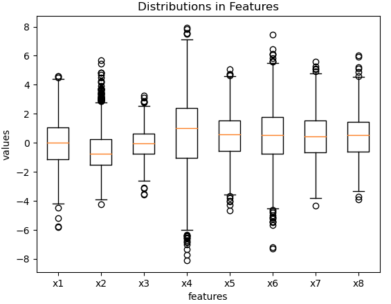
These distributions look reasonable, and show some variation among the different features.
Now we need to introduce some missing values. To do this, let’s define two functions for setting missing values in both the predictor and label values:
from random import choices
import numpy as np

def add_missing_values_to_X(X: np.array, n_nan: int=0) -> np.array:
    """
    Function to add missing values to predictor values X

    Inputs:
        X      -> set of predictor values
        n_nan  -> number of np.nan values to introduce
    Outputs:
        X with np.nan values introduced
    """
    # setup indices lists
    idx_x = [x_i for x_i in range(X.shape[0])]
    idx_y = [y_i for y_i in range(X.shape[1])]
    # add np.nan values
    idx_nan_x = choices(idx_x,k=n_nan)
    idx_nan_y = choices(idx_y,k=n_nan)
    X[idx_nan_x,idx_nan_y] = np.nan
    # return
    return(X)

def add_missing_values_to_y(y: np.array, n_nan: int=0) -> np.array:
    """
    Function to add missing values to label values y

    Inputs:
        y      -> set of label values
        n_nan  -> number of np.nan values to introduce
    Outputs:
        y with np.nan values introduced
    """
    # set type to float64
    y = y.astype('float64')
    # setup indices list
    idx = [x_i for x_i in range(y.shape[0])]
    # add np.nan values
    idx_nan = choices(idx,k=n_nan)
    y[idx_nan] = np.nan
    # return
    return(y)
Now we can proceed to introduce missing values, and then do a train-test split:
# add missing values to predictors
X = add_missing_values_to_X(X, n_nan=20)
# add missing values to labels
y = add_missing_values_to_y(y, n_nan=2)

# do train/test split
X_train, X_test, y_train, y_test = train_test_split(X, y, test_size=0.2, random_state=42)
In total, 20 missing values were inserted into the predictor features. Additionally, 2 more missing values were placed in the label column. Twenty percent of the data are then held-out as a test set.
Let’s see how our modified Decision Tree classifier performs on these data:
# declare the classifier and train the model
clf = DecisionTreeClassifier(max_depth=5, loss='gini')
clf.train(X_train,y_train)

# generate predictions
yp = clf.predict(X_test)

# evaluate model performance
idx    = ~np.isnan(y_test)
y_test = y_test[idx]
yp     = yp[idx]
print("accuracy: %.2f" % accuracy_score(y_test,yp))
print("precision: %.2f" % precision_score(y_test,yp))
print("recall: %.2f" % recall_score(y_test,yp))
accuracy: 0.86 precision: 0.85 recall: 0.89
Our implementation works, and yields good results. If you try to train the scikit-learn Decision Tree classifier on these data, you will see it generates a ValueError exception.
Regression Example with Missing Values
In the same manner as was done for the classification example, we can now try out the Decision Tree regressor implementation. Let’s start by creating a synthetic dataset with the make_regression function from scikit-learn:
# create a regression dataset
X,y = make_regression(n_samples=1000, n_features=8, n_informative=5, n_targets=1, noise=0.3, random_state=42)
Like before, these data consist of 1000 samples, with a total of 8 predictive features. Of these 8 features, only 5 are informative. We have a single target, and gaussian noise introduced with a standard deviation of 0.3.
To visualise what we have generated, let’s produce a box plot of the predictive features, as well as a histogram of the target:
# box plot of features
plt.boxplot(X)
plt.xlabel('features')
plt.ylabel('values')
plt.title('Distributions in Features')
plt.xticks([1, 2, 3, 4, 5, 6, 7, 8], ['x1', 'x2', 'x3', 'x4', 'x5', 'x6', 'x7', 'x8'])
plt.show()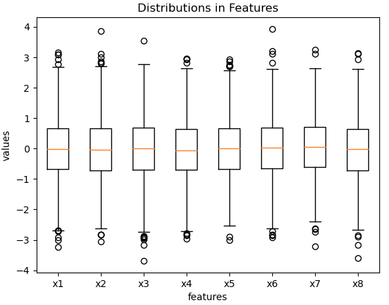
# histogram of label
plt.hist(y,bins=50)
plt.xlabel('y label')
plt.ylabel('frequency')
plt.title('Distribution in y Label')
plt.show()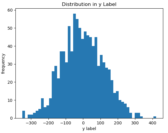
These data look reasonable, with significantly less variation in the predictor features when compared with the classification case.
Now we can proceed to introduce missing values, using the same two functions add_missing_values_to_X and add_missing_values_to_y defined previously. Following that, let’s do a train-test split:
# add missing values to predictors
X = add_missing_values_to_X(X, n_nan=5)
# add missing values to targets
y = add_missing_values_to_y(y, n_nan=2)

# do train/test split
X_train, X_test, y_train, y_test = train_test_split(X, y, test_size=0.2, random_state=42)
In total, 5 missing values were inserted into the predictor features. Additionally, 2 more missing values were placed in the target column. Twenty percent of the data is then held-out as a test set.
Let’s see how our modified Decision Tree regressor performs on these data:
# declare the regressor and train the model
rgr = DecisionTreeRegressor(max_depth=5, loss='mae', nans_go_right=False)
rgr.train(X_train,y_train)

# make predictions
yp = rgr.predict(X_test)

# evaluate model performance
idx    = ~np.isnan(y_test)
y_test = y_test[idx]
yp     = yp[idx]
print("rmse: %.2f" % np.sqrt(mean_squared_error(y_test,yp)))
print("mae: %.2f" % mean_absolute_error(y_test,yp))
rmse: 68.86 mae: 53.35
Our implementation works, and yields reasonable results. Note that in this case, I set the hyperparameter nans_go_right to False. If you try to train the scikit-learn Decision Tree regressor on these data, you will see it generates a ValueError exception.
Final Remarks
In this article you have learned:
- That Decision Trees can handle missing values in the data.
- One possible approach to how CART Decision Trees can be modified to handle missing values.
- An actual Python implementation of Decision Trees that can support missing values.
Please feel free to visit my GitHub page, where I have the complete Python code presented here in a single jupyter notebook. Download the notebook, and play around with the implementation. If you have any questions or comments, please leave them below!
Related Posts
Hi I'm Michael Attard, a Data Scientist with a background in Astrophysics. I enjoy helping others on their journey to learn more about machine learning, and how it can be applied in industry.
Hi There,
Can you please clarify what choices represent in your code? I tried to reproduce the code but got stuck here
Hi Nelly,
Thanks for your comment. The ‘choices’ function is imported from random, by: ‘from random import choices’. This wasn’t clear in the article, so I’ve updated it to make it more explicit. Note that the complete jupyter notebook for this article is available here: https://github.com/insidelearningmachines/Blog/blob/main/Notebook%20XVI%20Decision%20Trees%20with%20Missing%20Values.ipynb. If you have any further questions, please let me know!