Decision Trees are highly versatile, and form the basis of many powerful ensemble algorithms. However, they do posses many weaknesses as well. In this post, we will cover 8 key advantages and disadvantages of Decision Trees. Anyone wishing to make use of these models should be aware of these points.
Table of Contents
Video
If you prefer video content, please checkout my walk-through of this content on YouTube:
8 Advantages of Decision Trees
1. Relatively Easy to Interpret
Trained Decision Trees are generally quite intuitive to understand, and easy to interpret. Unlike most other machine learning algorithms, their entire structure can be easily visualised in a simple flow chart. I covered the topic of interpreting Decision Trees in a previous post.
2. Robust to Outliers
A well-regularised Decision Tree will be robust to the presence of outliers in the data. This feature stems from the fact that predictions are generated from an aggregation function (e.g. mean or mode) over a subsample of the training data. Outliers can start to have a bigger impact if the tree has overfitted. This topic was covered in a previous post.
3. Can Deal with Missing Values
The CART algorithm naturally permits the handling of missing values in the data. This enables us to implement a Decision Tree that does not require any additional preprocessing to treat for missing values. Most other machine learning algorithms do not have this capability. We implemented a Decision Tree that can handle missing values in a previous post.
4. Non-Linear
Decision Trees are inherently non-linear models. They are piece-wise functions of various different features in the feature space. As such, Decision Trees can be applied to a wide range of complex problems, where linearity cannot be assumed.
5. Non-Parametric
CART Decision Trees do not make assumptions regarding the underlying distributions in the data. This means we do not necessarily need to be concerned if the model is applicable to a given problem, given the assumptions of the algorithm. There are caveats to this, however, that will be discussed below (see point 4 in the disadvantages section).
6. Combining Features to Make Predictions
Combinations of features can be used in making predictions. The CART algorithm dictates that decision rules (which are if-else conditions on the input features) are combined together via AND relationships as one traverses the tree. This can be easily illustrated if we look at a Decision Tree trained on the Iris dataset:
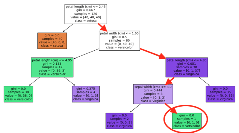
To arrive at the leaf node circled in red, we must follow the decision path highlighted by the red arrows. This decision path indicates that the following logic needs to play out, if we are to arrive that our selected leaf node:
- petal length > 2.45 and
- petal width > 1.65 and
- petal length <= 4.85 and
- sepal width > 3.0
Note the interdependence between the features. For example, the value of petal length will affect which feature we will look at next, and what condition we will apply to that feature. This enables complex interactions between features to be learned by the algorithm.
7. Can Deal with Categorical Values
The CART algorithm naturally permits the handling of categorical features in the data. This enables us to implement a Decision Tree that does not require any additional preprocessing (e.g. One-Hot-Encoding) to treat for categorical values. Most other machine learning algorithms do not have this capability. We implemented a Decision Tree to handle categorical features in a previous post.
8. Minimal Data Preparation
Minimal data preparation is required for Decision Trees. Since the training procedure in CART deals with each input feature independently, at each node in the tree, data scaling and normalisation are not required. In addition, it is also possible to implement Decision Trees that can handle missing values and categorical features, as discussed in points 3 & 7 above.
8 Disadvantages of Decision Trees
1. Prone to Overfitting
CART Decision Trees are prone to overfit on the training data, if their growth is not restricted in some way. Typically this problem is handled by pruning the tree, which in effect regularises the model. Care needs to be taken to ensure the pruned tree performs as we want on unseen data.
2. Unstable to Changes in the Data
Significantly different trees can be produced from training, if small changes occur in the data. As an example, let’s produce two datasets with only one point of difference:
# imports
import numpy as np
from sklearn.tree import DecisionTreeClassifier, plot_tree
from sklearn.datasets import make_classification

# make a dataset, and then introduce a change
X1,y1 = make_classification(n_samples=1000,
                            n_features=6,
                            n_informative=4,
                            n_classes=2,
                            shift=0.0,
                            scale=1.0,
                            random_state=42)

X2,y2 = make_classification(n_samples=1000,
                            n_features=6,
                            n_informative=3,
                            n_classes=2,
                            shift=0.0,
                            scale=1.0,
                            random_state=42)
The two datasets are identical, except X1 contains 4 informative features and X2 has only 3.
What kinds of trees will we get if we train on these two datasets?
# train the models
m1 = DecisionTreeClassifier(max_depth=3)
m1.fit(X1,y1)
m2 = DecisionTreeClassifier(max_depth=3)
m2.fit(X2,y2)

# plot tree 1
fig = plt.figure(figsize=(16,8))
_ = plot_tree(m1,
              filled=True,
              fontsize=10)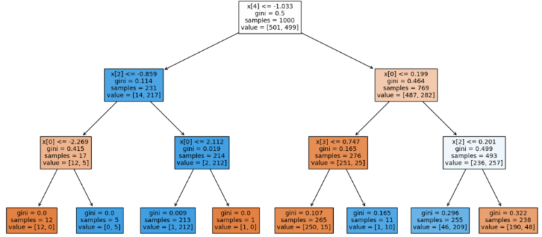
# plot tree 2
fig = plt.figure(figsize=(16,8))
_ = plot_tree(m2,
              filled=True,
              fontsize=10)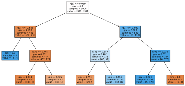
It is evident, looking at these two figures, that the learned tree structures are significantly different from each other. This aspect of Decision Trees potentially hurts explainability, especially to project stakeholders who are not data-savvy. This also implies that in a production environment, careful monitoring for changes in the input data needs to be in place.
3. Unstable to Noise
Similar to the previous point, Decision Trees are also sensitive to the presence of noise in the data. Let’s inject some noise into two of the input features X1 mentioned in point 2 above:
# box plot of the original features
plt.boxplot(X1)
plt.xlabel('features')
plt.ylabel('values')
plt.title('Distributions in Test Features with Outliers')
plt.xticks([1, 2, 3, 4, 5, 6], ['x1', 'x2', 'x3', 'x4', 'x5', 'x6'])
plt.show()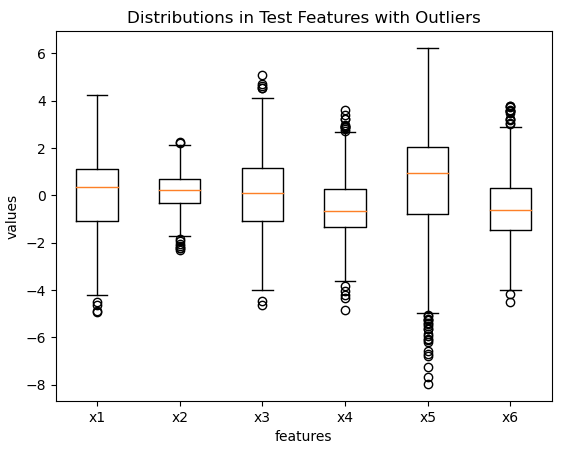
# alter 2 predictor features with some gaussian noise
X1_hat = np.copy(X1)
X1_hat[:,[0,5]] *= np.random.normal(size=(X1.shape[0],2))

# box plot of features
plt.boxplot(X1_hat)
plt.xlabel('features')
plt.ylabel('values')
plt.title('Distributions in Test Features with Outliers')
plt.xticks([1, 2, 3, 4, 5, 6], ['x1', 'x2', 'x3', 'x4', 'x5', 'x6'])
plt.show()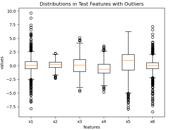
Some standard gaussian noise is introduced into features x1 and x6. Now let’s fit a Decision Tree classifier on the noisy data and view the structure of the model:
# train the model
m1 = DecisionTreeClassifier(max_depth=3)
m1.fit(X1_hat,y1)

# plot tree
fig = plt.figure(figsize=(16,8))
_ = plot_tree(m1,
              filled=True,
              fontsize=10)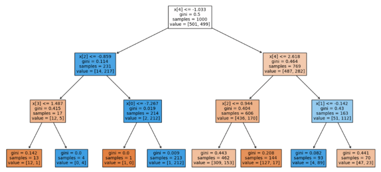
If we compare this Decision Tree structure with the one visualised for X1 (in point 2), we can see some significant changes. This highlights that the introduction, or presence, of noise in the data can result in different trees being produced. Like mentioned in the previous point, this can hurt explainability. It also implies that we should either monitor for noise in a production environment, or put in place steps to treat for noise in the data.
4. Non-Continuous
Decision trees are piece-wise functions, not smooth or continuous. This piece-wise approximation approaches a continuous function the deeper & more complex the tree gets. This however yields problems with overfitting (see point 1 above). Because of this, Decision Tree regressors tend to have limited performance, and are not good at extrapolation.
To visualise this, let’s imagine we have a dataset consisting of 1 informative predictor feature x, and 1 target y. Let’s make a scatter plot of the target versus our predictive feature:
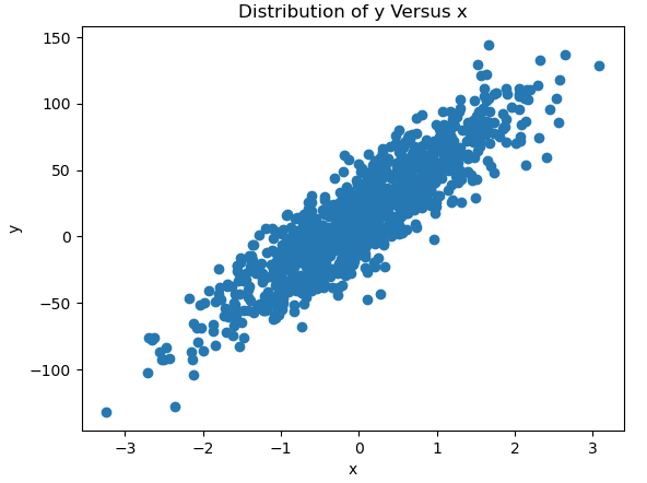
It is apparent from the figure that a linear relationship is present between x and y, plus some noise.
Now consider the case where a Decision Tree Regressor is trained on all the data where x \le 2. The remaining data (x \gt 2) is held out as a test set. Furthermore, let’s presume the maximum depth of the tree is set to 3. How well does the Decision Tree fit the training data? And how good is it on the test set?
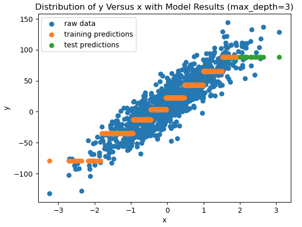
The piece-wise nature of the Decision Tree regressor is apparent in this plot. The orange points indicate how well the tree is approximating the training data. The limitations are obvious: this tree can only produce “steps” that roughly mimic the true linear relationship between x and y. Furthermore, the green points show us the prediction results. Since the tree was only trained on data where x \le 2, it is attempting to extrapolate over the test set. It is clear from the plot that the Decision Tree is unable to do so; the test set predictions are completely horizontal and do not follow the linear trend in the data.
We can attempt to improve this situation by increasing the complexity of the model. Let’s see the results again, but in this case for a tree with a maximum depth of 10:
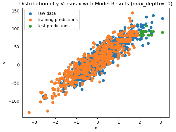
Now the piece-wise nature of the training results has disappeared, but it looks at though the model is attempting to fit the noise in the data. Ideally, we would expect a model to follow the linear trend in the data, and not attempt to reproduce the random fluctuations around this trend line. This plot suggests that our model has started to overfit on the training data. At the same time, the test set predictions remain horizontal, and do not follow the linear trend at all.
In this particular case, using a Linear Regression model would yield better results, since linearity is an inherent assumption in this algorithm. Since Linear Regression is a parametric algorithm, the model can make use of this assumption to extrapolate out to the test set.
5. Unbalanced Classes
Decision Tree classifiers can be biased if the training data is highly dominated by certain classes. Therefore, in situations where we are working with an unbalanced dataset, an additional preprocessing step will be needed to balance the data for training. Alternatively, if the implementation you are working with permits it, you can adjust weights within the model to account for class imbalances. The scikit-learn implementation supports this through the class_weight parameter.
6. Greedy Algorithm
CART follows a greedy algorithm, that finds only locally optimal solutions at each node in the tree. As such, the tree produced by the CART algorithm is a non-optimal global solution.
7. Computationally Expensive on Large Datasets
Decision Trees can become computationally expensive if there are many features to train on. Therefore, making use of a feature reduction technique as a preprocessing step may be required for very large datasets.
8. Complex Calculations on Large Datasets
One of the strengths of Decision Trees, mentioned earlier, is there interpretability. However, if the tree is unrestrained during training, or is trained on a large dataset, highly complex tree structures can result. For example, consider the two Decision Trees below:
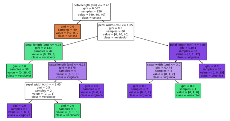
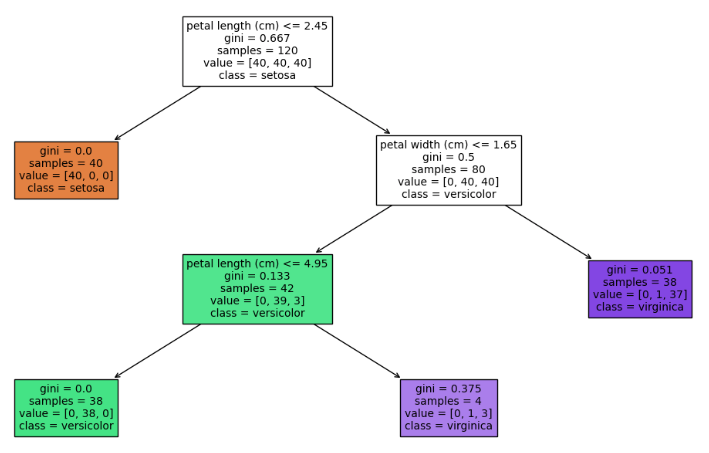
Both were trained on the Iris dataset, however the one on the left had no restrictions placed on it during training. The tree on the right was restricted in its growth during training. Comparing the two, it is clear that the simpler tree on the right is far easier to understand that the one on the left. Tree complexity only increases if an even larger dataset, with many more features, was used for training. All of this will tend to hurt interpretability.
Final Remarks
This article outlined 8 key advantages and disadvantages of Decision Trees. My intention here was to provide a summary of the strengths and weaknesses of this algorithm, to assist anyone interested in making use of it. I hope that you enjoyed this content, and gained some value from it. If you have any questions or comments, please leave them below!
Related Posts
Hi I'm Michael Attard, a Data Scientist with a background in Astrophysics. I enjoy helping others on their journey to learn more about machine learning, and how it can be applied in industry.

Software like many others lacks auto tune feature. The problems with auto tune software like H20 Flow or Search Grid and others is that they don exactly match hyperparameter used and or different options not/present in both software thus one can’t apply tuned value, like Using H2O Flow or MS NNi for Orange Data Mining thus useless. And with Orange one flying blind with hyperparameters. U cant proper train your models by guessing HP ! I don’t like cli versions either, is tedious, hard, different in code from one to another solutions provided, time consuming and repetitive tasks also the more the code, the more the sneaky logic and other errors due writing pages of code down. In many c cases u cant even apply it due not having particular support algorithm. Software that doesn’t have GUI and not AutoTune feature i do not even look ! That’s why i switched to one software to cover it all – MatLab ! Developers should wake up adding missing features and start thinking about ease of use ! U re just like Linux developers at the beginning everybody should use Linux in CLI ! Why do we not have DOS-OS any more ???