In this post, I will work through an implementation of K-Means from scratch in Python. We will start from first principals, and go straight through to coding a fully-functional K-Means model. Our code will then be tested against a toy dataset, and the results will be compared against those obtained from the K-Means available from scikit-learn.
Table of Contents
What is K-Means Clustering?
K-Means is an unsupervised learning algorithm, that aims to cluster input data based upon Euclidean distances. The number of clusters K must be input to the model, as the algorithm is incapable of finding this value on its own. The algorithm then proceeds to find the optimal cluster centres (i.e. the centroids), given the training data provided. Once the centroids are defined, all the input data can be assigned to a cluster based on their proximity to the centroids. In this way structure can be identified in the data, that might not be otherwise apparent.
The standard K-Means algorithm was first developed by Stuart Lloyd in 1957, as part of his work on pulse code modulation. These results were only published in 1982, due to limitations with the original work.
K-Means is a relatively simple non-parametric algorithm. As such, it yields results that can be easy to understand and interpret. However, this approach will perform poorly if key assumptions are not met, or the data is unsuitable for this technique. Please see the next section of this article for a complete list of assumptions and considerations regarding K-Means.
Assumptions and Considerations
The following key points will have to be kept in mind when clustering with K-Means:
- We will be making use of Euclidean distances. This will have the following impact on our approach:
- Clusters need to be ‘spherical’, meaning that the structure we are aiming to find can be discerned by how large (or small) the distance is alone. These distances are calculated from the cluster centroids to the data points. If this assumption is not met, transforming the data to another set of coordinates might be beneficial.
- Model performance will likely degrade in the case of high-dimensional data, as Euclidean distance becomes increasingly meaningless for higher dimensions. In these situations, applying a dimensionality reduction technique, as a preprocessing step, can help.
- Clusters are assumed to have similar sizes, meaning that no subset of clusters should have too few data points. If this assumption isn’t met, it is possible that the cluster assignments will not work as one would expect. Rerunning the algorithm multiple times, and selecting the centroid configuration that minimises our loss function, can help to avoid this situation.
- As already mentioned, the hyperparameter K will have to be determined prior to training the model. There are various techniques to accomplish this, such as the Elbow Method, Silhouette Method, etc.
Derivation of the K-Means Algorithm
We can start by visually describing the problem we are trying to solve. Consider the case where we have a 2-dimensional unlabelled dataset:
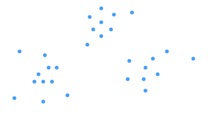
Figure 1: Scatter plot of a 2D unlabelled dataset.
Our objective is to find structure, if present, in these data. The ‘structure’ we are looking for in this case are clusters in the data. We can then provide labels to the data that indicate which cluster they belong to. Looking at Figure 1, it is apparent that the data points roughly fall into 3 groups. How can we identify these groups algorithmically?
Our first step is to select how many clusters we would like to search for. Let’s assume we correctly choose K=3. Next, we will need to identify the centres of each cluster. These centroids c_k are effectively the model parameters that we want to learn. Their positions are illustrated below:
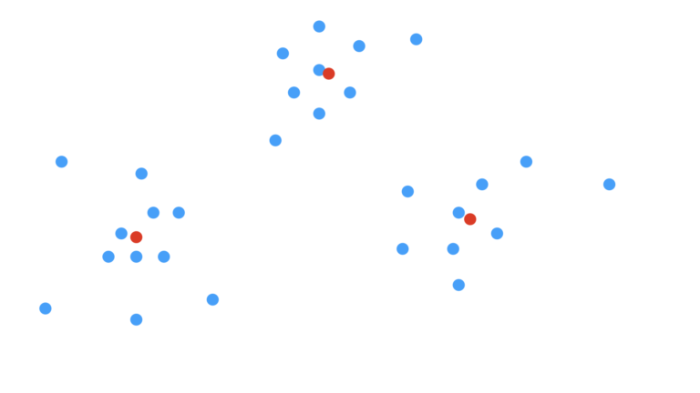
Figure 2: Scatter plot with cluster centroids included. The centroids are illustrated at red points.
With the centroids defined, we can now proceed to assign cluster labels to the data. These assignments will be based upon the Euclidean distance from each data point to each of the centroids. Figure 3 illustrates this comparison for the simplified case of a single data point:
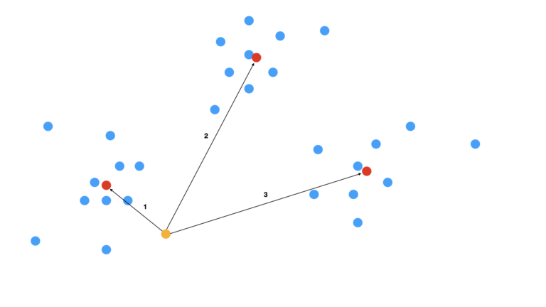
Figure 3: Scatter plot with comparison of centroids to an individual data point. The centroids are indicated in red, while the data point being examined is in orange. Numbered arrows indicate the distance of this data point to the first, second, and third centroids, respectively.
For the situation depicted in Figure 3, we can see that the data point is closest to the first centroid (the arrow numbered 1). As such, this data point is assigned to the first cluster. This procedure can be replicated to all the data, yielding cluster assignments for every single data point. The final outcome is shown in Figure 4:
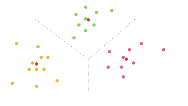
Figure 4: Scatter plot with final cluster assignments indicated by colour. Assignment to the first, second, and third clusters is labelled by orange, green, and pink, respectively. Centroids are also shown in red. Dotted lines indicate the rough partition of the data space found from clustering.
Figure 4 shows how the data have been grouped into 3 clusters, based on proximity to the centroids. Each individual data point is assigned to a cluster, and can thus be given a corresponding label.
Now that we have a clear idea of what our approach and objectives are, let’s describe in detail the standard K-Means algorithm for learning c_k:
- Set initial random values for the K centroids c_k.
- Assign each data sample x to a cluster. Select the cluster with the centroid that yields the smallest squared Euclidean distance: \text{argmin}_{c_k}\|x – c_k\|^2.
- Recalculate the positions of the K centroids, by computing the means of the assignments determined in step 2.
- Repeats steps 2. & 3. until either the centroid updates no longer produce meaningful changes, or a maximum number of iterations has been reached.
In practice, the 4-step procedure outlined above is repeated M times, and only the best model is selected. This is done to guard against finding only a locally optimal solution. We will compute the Total Within Cluster Sum of Squares (\text{WCSS}^{\text{tot}}) in order to compare the M different models:
\text{WCSS}^{\text{tot}} = \sum_k^K \text{WCSS}_k = \sum_k^K \sum_i^{N_k} \|x_i^{(k)} – c_k\|^2 (1)
where N_k is the number of samples in the kth cluster. The superscript over the sample x_i indicates this point is assigned to cluster k. The cluster configuration that minimises this function will be our selected model. Note that \text{WCSS}_k is the Within Cluster Sum of Squares for the kth cluster.
Build K-Means from Scratch in Python
We can now implement the algorithm, outlined in the previous section, into Python. Let’s start by loading in the necessary packages:
# imports
import numpy as np
from typing import Tuple, Dict
I will encapsulate all the necessary functionality within a single class. Let’s start with defining the initialiser and destructor functions:
class KMeans(object):
    """
    Class to encapsulate the K-Means algorithm
    """

    def __init__(self, K: int=3, n_init: int=10, max_iters: int=100) -> None:
        """
        Initialiser function for a class instance

        Inputs:
            K            -> integer number of clusters to assign
            n_init       -> integer number of times the algorithm will be applied when training
            max_iters    -> maximum number of iterations the algorithm is allowed to run before stopping
        """
        if K <= 0:
            raise ValueError(f'K must be a positive integer, got: {K}')
        if n_init <= 0:
            raise ValueError(f'n_init must be a positive integer, got: {n_init}')
        if max_iters <= 0:
            raise ValueError(f'Input argument max_iters must be a positive integer, got: {max_iters}')
        self.K          = K
        self.n_init     = n_init
        self.centroids  = np.array([])
        self.total_wcss = np.inf
        self.wcss_array = np.array([])
        self.max_iters  = max_iters

    def __del__(self) -> None:
        """
        Destructor function for class instance
        """
        del self.K
        del self.n_init
        del self.centroids
        del self.total_wcss
        del self.wcss_array
del self.max_iters- __init__(self, K, n_init, max_iters) : The initialiser is called when a class instance is created. Input arguments include:
- K, the integer number of clusters to search for. This was denoted as K above
- n_init, the integer number of times the algorithm will be rerun on the training data. This was denoted as M above
- max_iters, the maximum number of iterations permitted in the K-Means algorithm (step 4. of the previous section)
- __del__(self) : The destructor function used to release resources when a class instance is deleted.
The next functions will define how data samples are assigned to clusters, and how the training data is split accordingly:
    def __assign_samples(self, X : np.array, centroids : np.array) -> np.array:
        """
        Private function to assign samples to clusters

        Inputs:
            X -> numpy array of input features with shape: [number_samples, number_features]
            centroids -> numpy array of centroids with shape: [K, number_features]
        Output:
            numpy array indicating cluster assignment per sample with shape: [number_samples,]
        """
        # compute difference between input features & centroids through broadcasting
        differences = X[:,np.newaxis] - centroids[np.newaxis]
        # compute the squared euclidean distance for every (number_samples, K) pairs
        euclid_dist = np.einsum('ijk,ijk->ij', differences, differences)
        # find minimal distance for each sample & return
        return np.argmin(euclid_dist, axis=1)

    def __partition_data(self, X : np.array, cluster_assignment : np.array) -> list:
        """
        Private function to partition input features according to cluster assignment

        Inputs:
            X -> numpy array of input features with shape: [number_samples, number_features]
            cluster_assignment -> numpy array of cluser assignments with shape: [number_samples,]
        Output:
            list of numpy arrays of centroid for cluster, each array with shape:
            [cluster_number_samples, number_features]
        """
        # join features and cluster assignment
        X_assigned = np.concatenate((X, cluster_assignment.reshape(-1,1)),axis=1)
        # sort on the cluster assignment
        X_assigned = X_assigned[X_assigned[:, -1].argsort()]
        # partition the data based on the cluster assignment & return
return np.split(X_assigned[:,:-1], np.unique(X_assigned[:, -1], return_index=True)[1][1:])- __assign_samples(self, X, centroids) : This is a private function that assigns cluster labels to each row in the input data X. These assignments are based on the locations of the input centroids points. This function covers step 2. of the previous section.
- __partition_data(self, X, cluster_assignment) : Private function to split the input data X into a list with K elements. This split is based upon the input cluster_assignments, which is provided by the function __assign_samples.
The last private functions for our class will cover the calculation of \text{WCSS}^{\text{tot}} (see equation 1), and the centroid updates:
    def __compute_wcss(self, X : np.array, cluster_assignment : np.array,
                       centroids : np.array) -> Tuple[float, np.array]:
        """
        Private function to compute WCSS over all clusters

        Inputs:
            X -> numpy array of input features with shape: [number_samples, number_features]
            cluster_assignment -> numpy array of cluser assignments with shape: [number_samples,]
            centroids -> numpy array of centroids with shape: [K, number_features]
        Output:
            tuple containing the total WCSS, along with numpy array of WCSS values for clusters with shape: [K]
        """
        # break up the input features according to their cluster assignments
        X_clusters = self.__partition_data(X, cluster_assignment)
        # compute the WCSS for each cluster
        wcss_array = np.array([np.einsum('ij,ij', X_clusters[i] - centroids[i,:],
                                         X_clusters[i] - centroids[i,:]) for i in range(self.K)])
        # return the WCSS per cluster, along with the sum over all clusters
        return (np.sum(wcss_array), wcss_array)

    def __update_centroids(self, X : np.array, cluster_assignment : np.array) -> np.array:
        """
        Private function to update cluster centroids

        Inputs:
            X -> numpy array of input features with shape: [number_samples, number_features]
            cluster_assignment -> numpy array of cluser assignments with shape: [number_samples,]
        Output:
            numpy array of centroids with shape: [K, number_features]
        """
        # break up the input features according to their cluster assignments
        X_clusters = self.__partition_data(X, cluster_assignment)
        # compute new centroids & return
return np.array([np.mean(x, axis=0) for x in X_clusters])- __compute_wcss(self, X, cluster_assignment, centroids) : Private function to compute equation 1, based upon the input data X, cluster_assignment (provided by __assign_samples), and the centroids points. Returned is the total WCSS (\text{WCSS}^{\text{tot}}), along with the WCSS for each of the K clusters (\text{WCSS}_k).
- __update_centroids(self, X, cluster_assignment) : A private function to recalculate the centroid positions based upon the input data X and the cluster_assignment that was provided by __assign_samples. This function covers step 3. of the previous section.
We can now implement the training procedure for our class:
    def fit(self, X : np.array) -> None:
        """
        Training function for the class. Aims to find the optimal centroid values that minimise the WCSS

        Inputs:
            X -> numpy array of input features of assumed  shape [number_samples, number_features]
        """
        # initialise wcss score
        self.total_wcss = np.inf

        # loop over all iterations requested
        for _ in range(self.n_init):

            # initialise centroids
            centroids     = X[np.random.choice(X.shape[0], self.K, replace=False)]
            old_centroids = np.copy(centroids)
            # loop through the K-Means learning algorithm
            centroid_diff = np.ones((self.K))
            iteration     = 0
            while (not np.array_equal(centroid_diff,np.zeros(self.K))) and iteration < self.max_iters:
                # assign samples to clusters
                cluster_assignment = self.__assign_samples(X, centroids)
                # update centroids
                centroids = self.__update_centroids(X, cluster_assignment)
                # compute difference between centroids
                centroid_diff = np.abs(old_centroids - centroids)
                # increment counter & reset old_centroids
                iteration    += 1
                old_centroids = np.copy(centroids)

            # compute WCSS for the resulting clusters
            total_wcss, wcss_array = self.__compute_wcss(X, cluster_assignment, centroids)
            # check if we have a new optimal centroid configuration?
            if total_wcss < self.total_wcss:
                # if so, update storage objects
                self.total_wcss = total_wcss
                self.wcss_array = wcss_array
self.centroids = centroids- fit(self, X) : Public function to train the class instance on the input data X. This function implements the procedure outlined in the previous section in its entirety. Note that I have opted to stop training only when either the maximum number of iterations is reached (max_iters), or when the centroids no longer change at all. Some other implementations will make use of a tolerance threshold for the centroid changes, instead of insisting on zero difference.
The final functions for our class can now be defined:
    def predict(self, X : np.array) -> None:
        """
        Predict function for the class. Assigns cluster labels to each sample based on proximity to centroids

        Input:
            X -> numpy array of input features of assumed shape [number_samples, number_features]
        Output:
            numpy array indicating cluster assignment per sample with shape: [number_samples,]
        """
        if self.centroids.size == 0:
            raise Exception("It doesn't look like you have trained this model yet!")
        return self.__assign_samples(X, self.centroids)

    def return_wcss(self) -> Tuple[float, np.array]:
        """
        Public function to return WCSS scores (after training)

        Output:
            tuple containing the total WCSS, along with numpy array of WCSS values for clusters with shape: [K]
        """
        if self.centroids.size == 0:
            raise Exception("It doesn't look like you have trained this model yet!")
        return (self.total_wcss, self.wcss_array)

    def return_centroids(self) -> np.array:
        """
        Public function to return centroids (after training)

        Output:
            numpy array containing the centroids with shape: [K, number_features]
        """
        if self.centroids.size == 0:
            raise Exception("It doesn't look like you have trained this model yet!")
        return self.centroids

    def get_params(self, deep : bool = False) -> Dict:
        """
        Public function to return model parameters
        Inputs:
            deep -> boolean input parameter
        Outputs:
            Dict -> dictionary of stored class input parameters
        """
        return {'K':self.K,
                'n_init':self.n_init,
'max_iters':self.max_iters}- predict(self, X) : Public function to generate predictions on input data X. This function is essentially a wrapper around __assign_samples.
- return_wcss(self) : Public function to return the total WCSS (\text{WCSS}^{\text{tot}}), along with the WCSS for each of the K clusters (\text{WCSS}_k), found during training.
- return_centroids(self) : Public function to return the K centroids found during training.
- get_params(self, deep) : Public function used to return the instance input parameters. This is required for use with scikit-learn functionality.
Testing Performance
With our K-Means algorithm implemented, let’s now proceed to check how it performs on a toy dataset. Afterwards, we can compare how our custom implementation does versus the K-Means model available from scikit-learn.
To start, let’s import all the packages that are required, and then produce a dataset:
# imports
from sklearn.datasets import make_blobs
import matplotlib.pyplot as plt
from sklearn.metrics import mean_absolute_error, \
                            accuracy_score, \
                            precision_score, \
                            recall_score, \
                            f1_score

# produce dataset
X, y, centers = make_blobs(n_samples=1000, centers=3, n_features=2, return_centers=True, random_state=0)
I’m making use of the make_blobs function from scikit-learn to produce our data. These consist of 1000 samples and 2 features, grouped into 3 clusters. In addition, I request that the true centroids are returned so we can compare our modelling results against them later.
Let’s plot the data produced, and explicitly label the different clusters:
# visualise data
fig, ax    = plt.subplots(figsize=(10,8))
sc         = ax.scatter(X[:,0],X[:,1],c=y)
sc_centers = ax.scatter(centers[:,0],centers[:,1],c='r')
plt.xlabel('x1')
plt.ylabel('x2')
plt.title('Distribution of Data with True Cluster Assignments')
ax.legend(*sc.legend_elements(), title='clusters')
plt.show()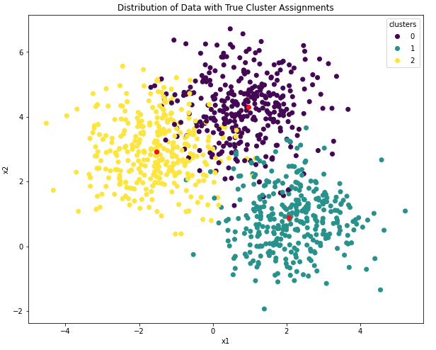
Figure 5: True distributions of clusters and centroid positions in the data. Centroids are indicated in red.
Membership to the different clusters is indicated by colour. In addition, the true cluster centroids are also illustrated. This figure represents the structure we are hoping to learn through K-Means.
Custom K-Means Model
We can make an attempt to learn the structure in our data, by applying our custom K-Means implementation defined previously. Let’s go ahead and declare an instance, train it, generate predictions, and plot the results:
# create an instance of KMeans
clt = KMeans(max_iters=300)

# fit the model to the data
clt.fit(X)

# obtain predictions
y_pred = clt.predict(X)

# obtain predicted centroids
centers_pred = clt.return_centroids()

# visualise predictions
fig, ax    = plt.subplots(figsize=(10,8))
sc         = ax.scatter(X[:,0],X[:,1],c=y_pred)
sc_centers = ax.scatter(centers_pred[:,0],centers_pred[:,1],c='r')
plt.xlabel('x1')
plt.ylabel('x2')
plt.title('Distribution of Data with Custom Predicted Cluster Assignments')
ax.legend(*sc.legend_elements(), title='clusters')
plt.show()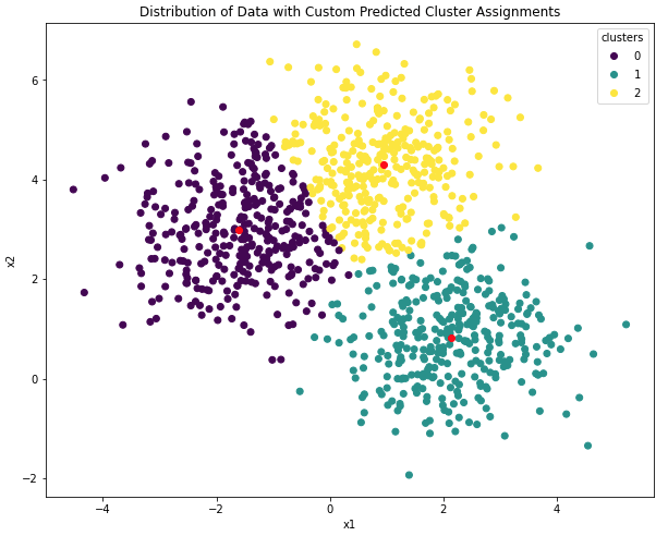
Figure 6: Centroid positions and cluster assignments from our custom K-Means implementation. Learned centroids are indicated in red.
This plot looks good! It appears our implementation has correctly identified the locations of the 3 clusters. Note that although the cluster labels are ordered differently here, when compared with Figure 5, the exact values of these labels are superficial. What is important is the grouping of the data samples, and centroid positions.
Let’s quantify how close the learned centroids are to the true values, by computing the mean absolute error (MAE) between the two:
# how accurate are our estimated centroids?
print(f'The mean absolute error between the predicted and true centroids is: {mean_absolute_error(centers,centers_pred[[2,1,0]]):.4f}')
The mean absolute error between the predicted and true centroids is: 0.0572
After accounting for the different labelling order, we get an MAE value of 0.0572. This is quite a nice result!
To get a sense for how well our K-Means model labelled the individual data points, let’s quantify the performance using standard metrics for classification problems:
# calibrate labelling
idx_0         = y_pred == 0
idx_1         = y_pred == 1
idx_2         = y_pred == 2
y_pred[idx_0] = 2
y_pred[idx_1] = 1
y_pred[idx_2] = 0

# how accurate are our cluster assignments?
acc = accuracy_score(y,y_pred)
pre = precision_score(y,y_pred,average='weighted')
rec = recall_score(y,y_pred,average='weighted')
f1  = f1_score(y,y_pred,average='weighted')
print(f'Accuracy score: {acc:.4f}')
print(f'Precision score: {pre:.4f}')
print(f'Recall score: {rec:.4f}')
print(f'F1 score: {f1:.4f}')
Accuracy score: 0.9180 Precision score: 0.9179 Recall score: 0.9180 F1 score: 0.9179
These results look good: the accuracy, precision, recall, and F1 scores are reasonably high. We should not expect these metrics to be 100%, since there is overlap between the clusters (as indicated in Figure 5). This overlap cannot be distinguished by K-Means.
Scikit-Learn K-Means Model
Now let’s compare the results above with those we can obtain with the scikit-learn implementation of K-Means. We can start by importing the model, training it, and then generating predictions:
# import scikit-learn K-Means
from sklearn.cluster import KMeans

# create an instance of KMeans
clt = KMeans(n_clusters=3, max_iter=300, random_state=0)

# fit the model to the data
clt.fit(X)

# obtain predictions
y_pred = clt.predict(X)
Like before, we can extract the learned centroids and plot the learned cluster distributions:
# obtain predicted centroids
centers_pred = clt.cluster_centers_

# visualise predictions
fig, ax    = plt.subplots(figsize=(10,8))
sc         = ax.scatter(X[:,0],X[:,1],c=y_pred)
sc_centers = ax.scatter(centers_pred[:,0],centers_pred[:,1],c='r')
plt.xlabel('x1')
plt.ylabel('x2')
plt.title('Distribution of Data with Scikit-learn Predicted Cluster Assignments')
ax.legend(*sc.legend_elements(), title='clusters')
plt.show()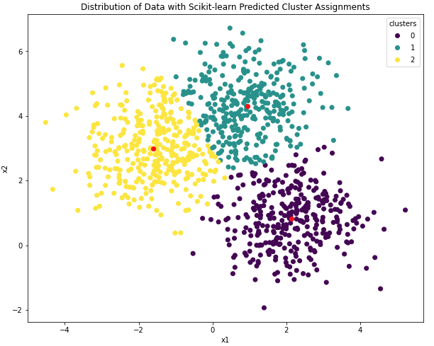
Figure 7: Centroid positions and cluster assignments from the scikit-learn K-Means model. Learned centroids are indicated in red.
Asides the different order in cluster labels, the plots in Figures 6 & 7 appear virtually identical. Let’s quantify the results obtained here in the same manner we did for our custom K-Means model:
# how accurate are our estimated centroids?
print(f'The mean absolute error between the predicted and true centroids is: {mean_absolute_error(centers,centers_pred[[1,0,2]]):.4f}')
The mean absolute error between the predicted and true centroids is: 0.0572
# calibrate labelling
idx_0         = y_pred == 0
idx_1         = y_pred == 1
idx_2         = y_pred == 2
y_pred[idx_0] = 1
y_pred[idx_1] = 0
y_pred[idx_2] = 2

# how accurate are our cluster assignments?
acc = accuracy_score(y,y_pred)
pre = precision_score(y,y_pred,average='weighted')
rec = recall_score(y,y_pred,average='weighted')
f1  = f1_score(y,y_pred,average='weighted')
print(f'Accuracy score: {acc:.4f}')
print(f'Precision score: {pre:.4f}')
print(f'Recall score: {rec:.4f}')
print(f'F1 score: {f1:.4f}')
Accuracy score: 0.9180 Precision score: 0.9179 Recall score: 0.9180 F1 score: 0.9179
These results are identical to those we obtained with our custom implementation, indicating that we’ve done a good job on our custom K-Means model.
Final Remarks
In this article you have learned:
- What the K-Means algorithm is, and when it was developed.
- The assumptions and considerations that need to be kept in mind when using the K-Means.
- A derivation of the K-Means algorithm.
- How to implement K-Means from scratch in Python.
- How our custom implementation of K-Means compares against the version available from scikit-learn.
I hope you enjoyed this article, and gained some value from it. If you would like to take a closer look at the code presented here, please take a look at my GitHub. If you have any questions or suggestions, please feel free to add a comment below. Your input is greatly appreciated.
Related Posts
Hi I'm Michael Attard, a Data Scientist with a background in Astrophysics. I enjoy helping others on their journey to learn more about machine learning, and how it can be applied in industry.