Neural Networks are machine learning models, that are structured in a way inspired by biological brains. Like their biological counterparts, Neural Networks are comprised of a collection of neurons, that individually perform basic information processing. Typically each neuron applies a simple non-linear function on the input received. Neurons work together within the network, passing information to each other in a structured way. The net effect is to yield a model that has significant potential to learn complex, non-linear relationships in the data.
Table of Contents

Neural Networks Explained Simply – image by Abi Plata
Why Neural Networks?
The fundament components to biological brains are neuron cells, which perform basic information processing tasks within animals. These cells are organised together into tissues and organs (e.g. brains), where the individual neurons are connected to each other in a ‘network’. The basic concept of this interconnected structure is shown in Figure 1 below:
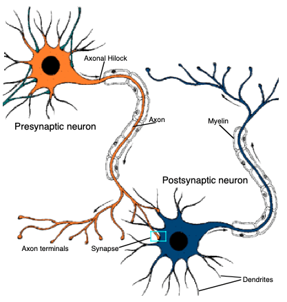
Figure 1: Two neuron cells connected to each other within a nervous tissue. Image by Jacques Sougné, University of Liège.
This figure illustrates just 2 neuron cells connected, whereas in reality there can be many more connections. As a result of this organisation, the individual cells are able to work together to yield a net processing capability that far exceeds that of any individual neuron.
Scientists and engineers were inspired by this example from nature. Starting in the 1940’s, work to develop artificial analogs to biological nervous tissue has been an area of active research. And this field continues to be very fluid to the present day (2023-06-21). New Neural Network architectures and models are regularly produced that push the boundaries of what is thought to be possible. The popularity of the ChatGPT Large Language Model (LLM), a type of Neural Network, is evidence of this.
Neural Networks are comprised of artificial neurons, that receive inputs \vec{x} and compute a response y. This response is typically a non-linear function of the inputs.
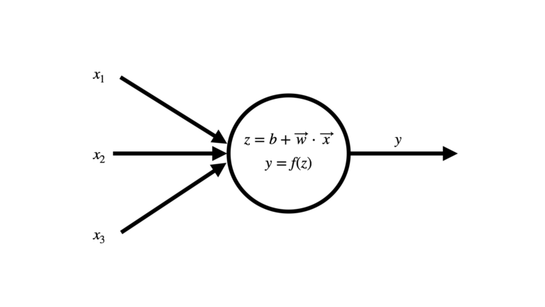
Figure 2: Artificial neuron in a Neural Network. Image by author.
The neuron receives input \vec{x} = \begin{bmatrix} x_1 \\ x_2 \\ x_3 \end{bmatrix} from either other neurons, or as input to the network. These inputs are weighted by \vec{w} = \begin{bmatrix} w_1 & w_2 & w_3\end{bmatrix}, and a bias b is added before applying an activation function f. Note that in Figure 2 we have the example of a neuron with only 3 inputs: in general this could be an arbitrary number.
The primary motivations for attempting to copy the structure of the brain are as follows:
- To understand how a biological brain actually works through computer simulation.
- To learn how the parallel computation, that biological brains are capable of, works.
- Produce practical machine learning models, that can handle complex tasks other learning algorithms are not capable of.
Despite these motivations, for decades the development and adoption of Neural Networks was impeded due to:
- Insufficient computational power available. This issue has been mitigated through continual advancements in computer processing power, as described by Moore’s Law.
- Insufficient data available. This problem has been resolved in part because of the resolution to point 1: increased computing power has enabled a plethora of digital devices to be developed. Just think of the Internet of Things (IoT) or smart phones. All of these digital devices collect data, meaning the amount of information available to train Neural Networks has exploded in the past decade.
Neural Networks typically out perform other machine learning algorithms when the amount of training data available becomes exceptionally large. What is “large” will depend on the nature of the specific problem. However a rough rule of thumb is that if a top-performing algorithm (e.g. Gradient Boost) does not show improved performance for increasing training set size, it may be a good idea to try a Neural Network instead.
However, training a Neural Network on these large datasets is also computationally intensive. Therefore for these algorithms to become competitive, both of the impediments mentioned above needed to be resolved. Now that this is generally the case, we can truly satisfy our third motivation: to build practical models that can handle complex tasks, no other learning algorithm can.
What are Neural Networks?
Neural Networks are collections of artificial neurons (see Figure 1 above) that function together to learn to solve a particular task. There are both supervised and unsupervised types of Neural Network architectures. As there are numerous examples of both types, with new ones being constantly developed, it is beyond the scope of this article to cover them all. Instead, I will go over both with a general illustrative example, that is representative of each group.
Supervised Neural Networks
With supervised learning, the training data consists of input predictor features \bold{X} = \begin{bmatrix} \vec{x_1} \\ \vec{x_2} \\ … \\ \vec{x_M}\end{bmatrix} and their associated labels y = [y_1, y_2, …, y_M]. In other words, the correct answers are known ahead of time, and we can use these to train our algorithm. Note that each \vec{x_i} is a row vector, and represents sample i out of the total M samples in the training data. Some of the most common and popular Neural Network architectures fall within this domain. Some examples of these include the Perceptron, Feedforward Neural Networks, Convolutional Neural Networks (CNN), and Recurrent Neural Networks (RNN). Most of these designs make use of backpropagation to update the model weights during training.
A representative example of a supervised Neural Network is shown in Figure 3 below:
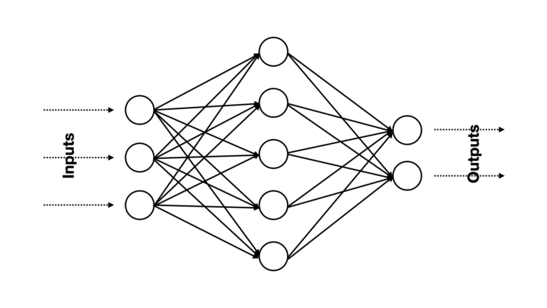
Figure 3: An example supervised Neural Network model. Predictor features enter on the left-hand side, and predictions are generated by the neurons on the right. Note that each circle represents an artificial neuron, and the solid arrows indicate the links, and direction of data flow, between different neurons in the network. Image by author.
There is a flow of information that propagates through the network from left to right. Data enters the network via the 3 neurons on the left-hand side, and the outputs from these neurons are then passed to 5 neurons in an intermediate group which do further processing. Finally, the outputs from the intermediate group are passed to the two neurons on the right-hand side, to yield an output. All of the connections (i.e. arrows) shown in this Figure are weighted, and these constitute the model parameters to learn (along with any biases).
The different groups of neurons at each stage within a Neural Network are termed layers. There can be an arbitrary number of layers within a Neural Network, however for the network shown in Figure 3 there are exactly three. Figure 4 highlights these different layers and how they are typically called:
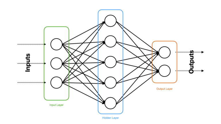
Figure 4: The same Neural Network explained in Figure 3, except the different layers are highlighted and labelled. Image by author.
There is exactly 1 Input Layer, 1 Hidden Layer, and 1 Output Layer. All supervised Neural Networks have exactly 1 input and output layers. However there are no restrictions on the number of hidden layers. The addition of hidden layers allows for more complex relationships to be found in the data, at the cost of making the model more computationally expensive, harder to interpret, and more prone to overfitting. In general, if a Neural Network has more than 1 hidden layer, it is termed a Deep Neural Network.
The number of neurons in the input layer are restricted by the number of features in our data. Normally, there is 1 input neuron for each input feature in the data. The number of neurons in the output layer is also constrained by the nature of the desired predictions, i.e. if we are solving a binary classification problem, a single sigmoid neuron in the output layer would do. The hidden layers do not have hard restrictions on the number of neurons permitted.
However, we must keep in mind that adding neurons in the hidden layer(s) also means we are adding model parameters, which increases the chance of overfitting. Ideally, a hyperparameter tuning stage should be added to our analysis to determine the optimal number of layers, and neurons per layer, for our model.
Unsupervised Neural Networks
With unsupervised learning, the training data consists solely of input features \bold{X} = \begin{bmatrix} \vec{x_1} \\ \vec{x_2} \\ … \\ \vec{x_M}\end{bmatrix}, where \vec{x_i} is a row vector representing sample i out of the total M samples. The aim of this type of learning is to try to identify structure in the data. Clustering is a common task that falls within the unsupervised learning domain.
There are a variety of different approaches to doing unsupervised learning with Neural Networks. Autoencoders and Generative Adversarial Networks (GANs) make use of backprogation, and have architectures that superficially resemble those depicted in Figures 3 & 4. Autoencoders can be used for data compression or dimension reduction, whereas GANs are used for generating data from learned patterns in a training data set.
Self Organising Maps (SOPs) are another type of unsupervised Neural Network that makes use of competitive learning. These models are a popular choice for data compression or dimension reduction. Like autoencoders, they provide a means by which data can be compressed without the linearity assumption that is central to PCA.
Finally, there are also Energy-Based Neural Networks that are used for unsupervised tasks. These models make use of stochastic binary neurons, and have learning algorithms that aim to minimise an energy function given the observed data. Restricted Boltzmann Machines (RBMs) and Deep Belief Networks (DBNs) are examples of this type of model, and like GANs are generative algorithms.
For the purpose of this article, I will focus a bit more on the energy-based model architecture. A representative example of this type of unsupervised Neural Network is shown in Figure 5 below:
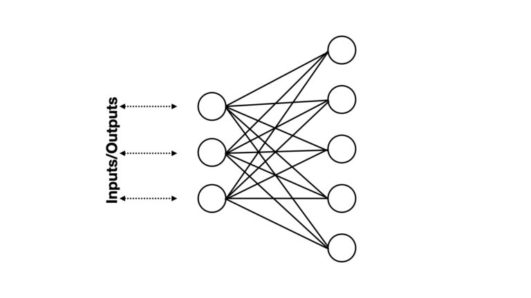
Figure 5: An example energy-based unsupervised Neural Network. Data flows into, and out from, the three neurons on the left. The neurons on the right do not directly interact with the outside. Note that each neuron applies a stochastic binary activation function. Image by author.
Some notable differences can be seen when comparing the architecture in Figure 5 versus that shown in Figure 3. First, only one set of neurons interacts with the external world. The other set remains isolated within the network. Individual neurons are connected with one another, represented by solid lines (no arrow) to indicate that information can flow back-and-forth within this structure.
We can assign neurons to specific layers within this network, in the same manner as we did for the supervised example. Let’s illustrate this in Figure 6:
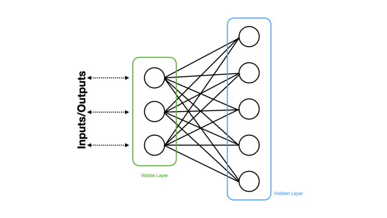
Figure 6: The same Neural Network illustrated in Figure 5, except the different layers are highlighted and labelled. Image by author.
Here we can see that there are exactly two layers within this network. The Visible Layer consists of all the neurons which interact with the outside world, while the Hidden Layer comprises all the neurons which have no direct external connection. The neurons in the visible layer can also be termed Visible Units, while the neurons in the hidden layer can be called Hidden Units.
The number of neurons per layer can vary, like in the supervised example. The number of visible units will be generally restricted to the number of features in the data, whereas no hard restrictions exist for the hidden units. We must be careful to not add too many hidden units however, in case of overfitting.
The number of hidden layers can vary, whereas there is always only one visible layer. The illustrations in Figures 5 & 6 are representative of a RBM, where only one hidden layer is present. Multiple hidden layers are consistent with DBNs.
General Considerations when Using Neural Networks
There are a few key points to keep in mind if you’re interested in using a Neural Network algorithm:
- Neural Networks come into their own when trained on very large datasets, where more traditional machine learning algorithms are unable to exploit the available information.
- Non-Linear relationships should be expected. Neural Networks excel at building non-linear mappings of data. If your particular problem happens to be linear in nature, you should not use a Neural Network.
- As Neural Networks can be very large and complex, sufficient computing power will need to be available to make your model train in a reasonable amount of time. This is compounded by the fact that the training data will also need to be sufficiently large as well (see point 1.).
- Neural Networks are typically treated as black boxes, due to the fact that their internal structure is highly complex. Explaining why your model produces certain output, to stakeholders, can be more difficult when compared with other machine learning algorithms.
Final Remarks
This article outlined a general introduction into Neural Networks, and the various different architectures that are used to build these models. This is a very extensive family of machine learning algorithms, and so the content here is by no means exhaustive. My hope was to provide the reader with an opportunity to “get their feet wet” on this subject, and in this way have Neural Networks explained to a very basic level. I hope you enjoyed this content, and gained some value from it. If you have any questions or comments, please leave them below!
Related Posts
Hi I'm Michael Attard, a Data Scientist with a background in Astrophysics. I enjoy helping others on their journey to learn more about machine learning, and how it can be applied in industry.