In this article, we will implement a Multilayer Perceptron Classifier from scratch. Instead of making use of a framework such as TensorFlow or Pytorch, we’ll build our model from the ground-up. The sole dependancy we will rely on is the popular Numpy package for numerical computations. By working through this exercise, we will gain a deeper insight into how these powerful algorithms actually work.
Table of Contents

Build a Multilayer Perceptron Classifier with Numpy – image by author
Video
For those who prefer video content, you can watch me work through the example in this article here:
Model Description
In a previous post, I covered how to build a multilayer perceptron regressor with numpy. The model we will build here is analogous to this previous article, except that now we will aim to solve binary classification problems, instead of regression. As such, the type of Neural Network we will implement is a Multilayer Perceptron Classifier, also known as a Feedforward Neural Network Classifier.
At a high level, the architecture of the Neural Network we will build is illustrated in Figure 1:
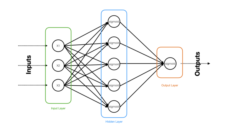
Figure 1: Schematic of the 3-layer Neural Network Classifier to be built. Input, hidden, and output layers are highlighted, and the relevant activation functions are written within each neuron.
The densely connected Neural Network illustrated in Figure 1 consists of 3 layers: a input, hidden, and output layer. The raw input predictor features (x1, x2, x3) are clamped to the input layer, that distributes these features to the hidden layer. Sigmoid activation functions are applied to the neurons within the hidden and output layers. Five neurons makeup the hidden layer, while a single neuron constitutes the output layer. With this setup, our network is applicable to learn binary classification problems.
At a high level, the learning procedure will follow this sequence of steps:
- \text{for e} = 1..epochs:
- Do a Forward Pass
- Do a Backward Pass
- Update the model weights
I covered the technical details involved with the learning procedure in an earlier article, however there I focused on a model designed to handle regression. For a classifier, some details will change. In particular, our choice of loss function will be cross entropy:
\ell(y^{true},y^{pred}) = -y^{true} log_2 (y^{pred}) -(1.0-y^{true}) log_2 (1.0-y^{pred}) (1)
Note that form of (1) is specific for binary classification problems, i.e. y^{true} \in (0.0, 1.0). In addition to the different loss function, the activation function in the output layer will be a sigmoid (rather than linear). Therefore we’ll need to take this into account when implementing the forward and backward passes. In particular, we need to take note of the following:
\frac{\partial \ell}{\partial y^{pred}} = -\frac{1}{ln2}\lbrack \frac{y^{true}}{y^{pred}} – \frac{1 – y^{true}}{1-y^{pred}}\rbrack (2)
\frac{df}{dz^2} = y^{pred} (1 – y^{pred}) (3)
where z^2 is the input to the activation function f in the output layer.
For the sake of simplicity, the Backward Pass will make use of backpropagation with batch gradient descent. As such, we will only need to iterate through our training procedure for the number of epochs desired (as all the training data will be applied when updating the weights at each iteration).
Generating predictions will involve a single Forward Pass, with a trained model, on a set of input predictor features.
Implementation of a Multilayer Perceptron Classifier
Let’s now implement our classifier. I will be focusing exclusively on the Python coding here, so if you’re interested in more of the mathematical details please refer to my previous article on how Neural Networks learn. When reviewing that article, please keep in mind the discussion in the previous section of this post.
We can start by importing all the necessary packages:
# imports
from typing import List, Tuple
import numpy as np
from sklearn.datasets import make_classification
from sklearn.model_selection import train_test_split
from sklearn.metrics import accuracy_score, f1_score
import matplotlib.pyplot as plt
Our implementation will be encapsulated within a class called MLP351Classifier. Its structure will be exactly the same as the network in Figure 1. Let’s start with the class definition:
class MLP351Classifier(object):
    """
    Class to encapsulate a Multilayer Perceptron / FeedForward Neural Network classifier
    """

    def __init__(self, lr: float=1e-2, epoches: int=100) -> None:
        """
        Initialiser function for a class instance

        Inputs:
            lr      -> learning rate
            epoches -> number of epoches to use during training
        """
        self.lr      = lr
        self.epoches = epoches
        self.layers  = [3,5,1]
        self.weights = []
        self.biases  = []
        self.loss    = []

    def __del__(self) -> None:
        """
        Destructor function for a class instance
        """
        del self.lr
        del self.epoches
        del self.layers
        del self.weights
        del self.biases
        del self.loss
Next we can proceed to implement protected functions for the loss (1) and it’s derivative (2):
    def _loss(self, y_true: np.array, y_pred: np.array) -> np.array:
        """
        Function to compute cross-entropy loss per sample

        Inputs:
            y_true -> numpy array of true labels
            y_pred -> numpy array of prediction values
        Output:
            loss value
        """
        return -y_true*np.log2(y_pred) - (1 - y_true)*np.log2(1 - y_pred)

    def _derivative_loss(self, y_true: np.array, y_pred: np.array) -> np.array:
        """
        Function to compute the derivative of the cross-entropy loss per sample

        Inputs:
            y_true -> numpy array of true labels
            y_pred -> numpy array of prediction values
        Output:
            loss value
        """
        return -(1/np.log(2))*( (y_true/y_pred) - ((1-y_true)/(1-y_pred)) )
The sigmoid function, and its derivative (3), can also be placed within protected functions:
    def _sigmoid(self, z: np.array) -> np.array:
        """
        Function to compute sigmoid activation function

        Input:
            z -> input dot product w*x + b
        Output:
            determined activation
        """
        return 1/(1+np.exp(-z))

    def _derivative_sigmoid(self, z: np.array) -> np.array:
        """
        Function to compute the derivative of the sigmoid activation function

        Input:
            z -> input dot product w*x + b
        Output:
            determined derivative of activation
        """
        return self._sigmoid(z)*(1 - self._sigmoid(z))
We can now start to bring these pieces together. I’ll implement two further protected functions, that will take care of a single forward pass, and backward pass, during training:
    def _forward_pass(self, X: np.array) -> Tuple[List[np.array], List[np.array]]:
        """
        Function to perform forward pass through the network

        Input:
            X -> numpy array of input predictive features with assumed shape [number_features, number_samples]
        Output:
            list of activations & derivatives for each layer
        """
        # record from input layer
        input_to_layer = np.copy(X)
        activations    = [input_to_layer]
        derivatives    = [np.zeros(X.shape)]

        # hidden layer
        z_i = np.matmul(self.weights[0],input_to_layer) + self.biases[0]
        input_to_layer = self._sigmoid(z_i)
        activations.append(input_to_layer)
        derivatives.append(self._derivative_sigmoid(z_i))

        # output layer
        z_i = np.matmul(self.weights[1],input_to_layer) + self.biases[1]
        input_to_layer = self._sigmoid(z_i)
        activations.append(input_to_layer)
        derivatives.append(self._derivative_sigmoid(z_i))

        # return results
        return(activations, derivatives)

    def _backward_pass(self,
                       activations: List[np.array],
                       derivatives: List[np.array],
                       y: np.array) -> Tuple[List[np.array], List[np.array]]:
        """
        Function to perform backward pass through the network

        Inputs:
            activations -> list of activations from each layer in the network
            derivatives -> list of derivatives from each layer in the network
            y           -> numpy array of target values
                           with assumed shape [number_samples, output dimension]
        Output:
            list of numpy arrays containing the derivates of the loss function wrt layer weights
        """
        # record loss
        self.loss.append((1/y.shape[1])*np.sum(self._loss(y, activations[-1])))

        # output layer
        dl_dy2 = self._derivative_loss(y, activations[2])
        dl_dz2 = np.multiply(dl_dy2, derivatives[2])
        dl_dw2 = (1/y.shape[1])*np.matmul(dl_dz2, activations[1].T)
        dl_db2 = (1/y.shape[1])*np.sum(dl_dz2, axis=1)

        # hidden layer
        dl_dy1 = np.matmul(self.weights[1].T, dl_dz2)
        dl_dz1 = np.multiply(dl_dy1, derivatives[1])
        dl_dw1 = (1/y.shape[1])*np.matmul(dl_dz1, activations[0].T)
        dl_db1 = (1/y.shape[1])*np.sum(dl_dz1, axis=1)

        # return derivatives
        return([dl_dw1, dl_dw2], [dl_db1, dl_db2])
The final protected function will be responsible for updating the weights, and biases, during training:
    def _update_weights(self, dl_dw: List[np.array], dl_db: List[np.array]) -> None:
        """
        Function to apply update rule to model weights

        Input:
            dl_dw -> list of numpy arrays containing loss derivatives wrt weights
        """
        self.weights[0] -= self.lr*dl_dw[0]
        self.weights[1] -= self.lr*dl_dw[1]
        self.biases[0]  -= self.lr*dl_db[0].reshape(-1,1)
        self.biases[1]  -= self.lr*dl_db[1].reshape(-1,1)
We now have all the tools in place to implement the public functions for this class. This will consist of a fit function, for training the model, and a predict function, for generating predictions after training:
   def fit(self, X: np.array, y: np.array) -> None:
        """
        Function to train a class instance

        Inputs:
            X -> numpy array of input predictive features with assumed shape [number_samples, number_features]
            y -> numpy array of target values with assumed shape [number_samples, output dimension]
        """
        # initialise the model parameters
        self.weights.clear()
        self.biases.clear()
        self.loss.clear()
        for idx in range(len(self.layers)-1):
            self.weights.append(np.random.randn(self.layers[idx+1], self.layers[idx]) * 0.1)
            self.biases.append(np.random.randn(self.layers[idx+1], 1) * 0.1)
        # loop through each epoch
        for _ in range(self.epoches):
            # do forward pass through the network
            activations, derivatives = self._forward_pass(X.T)
            # do backward pass through the network
            dl_dw, dl_db = self._backward_pass(activations, derivatives, y.T)
            # update weights
            self._update_weights(dl_dw, dl_db)

    def predict(self, X: np.array) -> np.array:
        """
        Function to produce predictions from a trained class instance

        Input:
            X -> numpy array of input predictive features with assumed shape [number_samples, number_features]
        Output:
            numpy array of model predictions
        """
        # do forward pass through the network
        activations, _ = self._forward_pass(X.T)
        # return predictions
        return np.rint(activations[2]).reshape(-1)
Create a Toy Dataset
Let’s produce a small dataset with make_classification from scikit-learn. These data will consist of 10000 samples, with 3 predictive input features. Of these features, 2 will be informative while 1 will be redundant. Our target will be binary (0.0,1.0):
# generate a dataset
X,y = make_classification(n_samples=10000, n_features=3, n_informative=2, n_redundant=1, random_state=42)
We can produce a box plot to get a sense of the distribution in the input predictive features:
plt.boxplot(X)
plt.title("Distribution of Input Predictive Features")
plt.xlabel("feature")
plt.ylabel("input unit")
plt.show()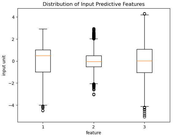
Figure 2: Distribution of the 3 input predictive features for our classifier.
The generated targets can be illustrated with a histogram:
plt.hist(y)
plt.title("Distribution of Labels")
plt.xlabel("class")
plt.ylabel("output unit")
plt.show()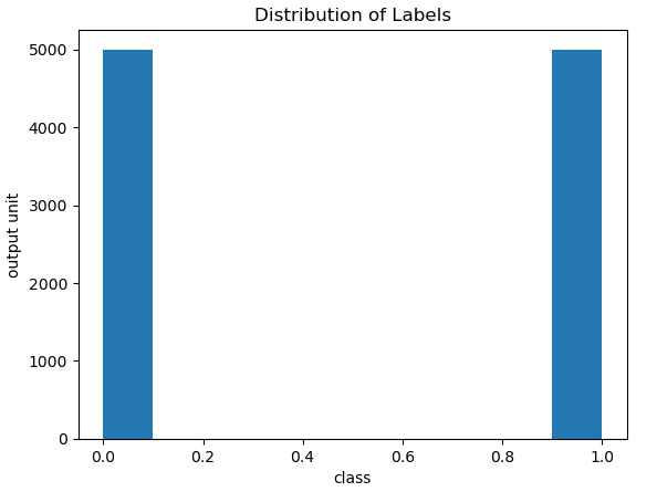
Figure 3: Histogram plot of the two class labels (0.0, 1.0) in our dataset.
Referring to Figure 2: the input features 2 & 3 appear to be approximately zero-centered, whereas feature 1 has a positive-valued median. The range for each feature varies, with the narrowest belonging to feature 2 (-2,+2) and the broadest with feature 3 (-4, +4). Outliers are present for each feature, with the largest concentration being with feature 2.
Referring to Figure 3: there appears to be no class imbalance in these data.
Finally, we can do a train-test split, with 80% of the data being allocated for training:
# perform train-test split
X_train, X_test, y_train, y_test = train_test_split(X, y, test_size=0.2, random_state=42)
Test our Multilayer Perceptron Classifier
We’re now ready to test out our custom Neural Network classifier! Let’s create an instance of MLP351Classifier, and train it on the appropriate data. I’ll make use of a learning rate of 1.0 and we will train for 2000 epochs:
# train the classifier
model = MLP351Classifier(lr=1.0,epoches=2000)
model.fit(X_train,y_train.reshape(-1,1))
Plotting the training loss will reveal if our model is functioning as expected:
# plot the training loss
plt.plot(model.loss)
plt.title("Training Loss")
plt.xlabel("epochs")
plt.ylabel("loss")
plt.show()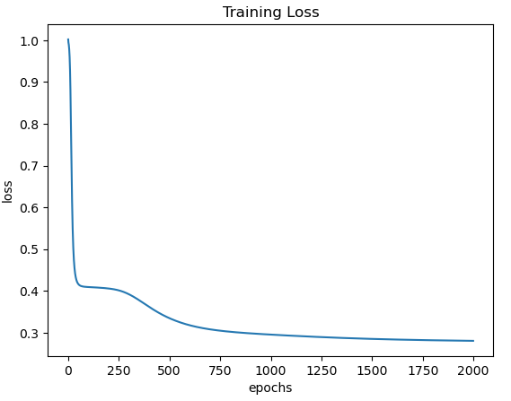
Figure 4: Training loss as a function of epochs.
Figure 4 shows a rapid decline at first, followed by a gradual decline for ~500 epochs. The loss then gentily slopes down from epoch 500 to 2000. This indicates that our training procedure is working. Now let’s evaluate how well our classifier performs in making predictions:
# generate predictions
y_pred = model.predict(X_test)

# evaluate model performance
print(f"accuracy: {accuracy_score(y_test, y_pred):.2f} and F1 score: {f1_score(y_test, y_pred):.2f}")
accuracy: 0.93 and F1 score: 0.93
The accuracy and F1 results indicate that our classifier functions reasonably well on the test data provided.
Final Remarks
In this post we have covered:
- The general architecture of a Multilayer Perceptron Classifier.
- How to implement a Multilayer Perceptron Classifier from scratch just using numpy.
- How to test our implementation to confirm that it works.
I hope you enjoyed this article, and gained some value from it. If you would like to take a closer look at the code presented here, please take a look at my GitHub. If you have any questions or suggestions, please feel free to add a comment below. Your input is greatly appreciated.
Related Posts
Hi I'm Michael Attard, a Data Scientist with a background in Astrophysics. I enjoy helping others on their journey to learn more about machine learning, and how it can be applied in industry.
Thank you very much for this article, I had been looking around for something that would make me understand Neural networks from scratch, and not hide all the fancy stuff behind libraries.