In this post, I will cover the Backpropagation algorithm. This procedure makes use of gradient descent, and the chain rule of calculus, to determine the update rules for all the weights within a Neural Network. This is done with respect to the loss computed between model output and true label values. The importance of this algorithm cannot be understated in the field of machine learning. Its adoption facilitated the development of supervised Neural Networks with many hidden layers, and thereby led directly to the rise of modern Deep Learning models.
Table of Contents

Understanding Backpropagation – image by Abi Plata
Why do we need Backpropagation?
Backpropagation arose out of the desire to have self-organising Neural Networks. In other words, to have nets that are capable of learning interesting features from the raw input data. In my article on the Perceptron, we saw that these simple Neural Networks require a set of hand-made input features in order to work. Our aim here is to move away from this dependancy. This will be achieved by adding hidden layers to our network, such that they can learn the representations required by the output layer.
The challenge then becomes: how to we learn the weights on these hidden layers? This is where the Backpropagation algorithm comes into play.
When was Backpropagtion Developed?
The terminology of “Backpropagation” was first developed by Frank Rosenblatt in his 1962 paper Principles of Neurodynamics. A first working example, of a multi-layered Neural Network making use of this technique, was demonstrated by Amari Shun’ichi in his 1967 paper A Adaptive Theory of Pattern Classifiers. Backpropagation was popularised by the 1986 paper Learning Representations by Backpropagating Errors by David Rumelhart, Geoffrey Hinton, and Ronald Willams.
How does Backpropagation Work?
The learning procedure for a supervised Neural Network consists of 2 parts: a forward pass and backward pass. The forward pass always precedes the backward pass, and these passes are typically repeated a number of times over the training data. Let’s now look into each more closely.
Forward Pass
The forward pass involves applying the predictor features \vec{x} in our training data to the input layer of the Neural Network. Activations from this layer \vec{y}^1 are passed as inputs to the second layer, where further activations \vec{y}^2 are computed. This process continues until we arrive at the output layer of the net, where the final predictions \vec{y}^{pred} are determined. Figure 1 illustrates this process:
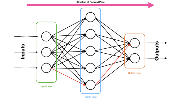
Figure 1: Depiction of a Neural Network with a single input, hidden, and output layers. Data passes from the input to the output layer, via the hidden layer. The direction of data flow is indicated by the pink arrow on the top of the figure. The connections between individual neurons are also indicated. One possible path through the network is highlighted by the arrows in red.
Note that for layer i, the associated activations are computed by making use of an activation function f in the following manner:
z^i_j = b^i_j + \vec{w}^i_j \cdot \vec{y}^{i-1} (1)
y^i_j = f(z^i_j) (2)
where the above calculations are done element-wise for each neuron j in layer i: \vec{y}^i = [y^i_1, y^i_2, …]. The weights \vec{w}^i_j and bias b^i_j are specific for each neuron in the layer. The input to this particular neuron \vec{y}^{i-1} is the output from the previous layer i-1, or the raw input data if i=1.
Backward Pass
After a forward pass, we have a set of prediction values \vec{y}^{pred} for the input \vec{x}. We are now confronted with the task of updating our model parameters \vec{w}^i_j and b^i_j.
The general idea is to compute the loss \ell at the output layer, and then propagate the effects of this loss back towards the input layer. As we traverse backwards, we can compute how best to update the weights by making use of gradient descent. Figure 2 visualises this idea:
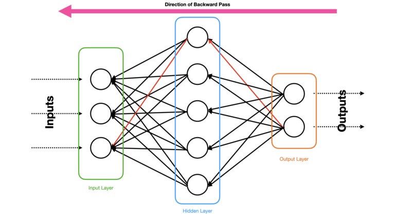
Figure 2: Depiction of a Neural Network with the same architecture as in Figure 1. The effect of the error between \vec{y}^{pred} and \vec{y}^{true} pass from the ouput to the input layer, via the hidden layer. The direction of data flow is indicated by the pink arrow on the top of the figure. The connections between individual neurons are also indicated. One possible path through the network is highlighted by the arrows in red.
Notice the arrows connecting different neurons are flipped with respect to Figure 1, indicating the change in direction of information flow. The Backpropagation procedure we will undertake is as follows:
- Compute the loss for the values produced at the output layer \vec{y}^{pred} compared with the true labels \vec{y}^{true}: \ell = \ell(\vec{y}^{pred}, \vec{y}^{true}). The loss \ell needs to be a differentiable function of y^{pred} (see step 2.)
- Calculate the partial derivative of the loss with respect to the predicted values: \partial\ell / \partial y^{pred}
- Use the chain rule to determine \partial\ell / \partial z^i = (\partial\ell / \partial y^{pred})(df / dz^i). For the specific case where y^i = y^{pred}, the index i refers to the output layer of the network. We will assume that df / dz^i is known, and this tells us how a change in inputs to the layer affect the loss \ell
- Note from equation (1) that z^i = \vec{w}^i \cdot \vec{y}^{i-1} (I will drop the subscript j). Therefore \partial \ell / \partial w^i = (\partial\ell / \partial z^i)(\partial z^i / \partial w^i) = (\partial\ell / \partial z^{i})y^{i-1}
- To workout \frac{\partial\ell}{\partial b^i}, the chain rule shows: \frac{\partial\ell}{\partial b^i} = \sum^N \frac{\partial \ell}{\partial z^i} , where N is the number of samples used during the forward/backward pass
- To work out \partial\ell / \partial y^{i-1}, we again apply the chain rule: \partial\ell / \partial y^{i-1} = (\partial\ell / \partial z^i)(\partial z^i / \partial y^{i-1}) = (\partial\ell / \partial z^i)w^i. This value needs to be summed over all connections from i-1 to i
- Using the result from 5., we can then propagate back to layer i-2, starting at step 2. above, replacing \partial\ell / \partial y^{pred} with \partial\ell / \partial y^{i-1}
At each layer, the update to the weights and biases can be made using a simple gradient decent rule:
\Delta w = -\epsilon\frac{1}{N}\frac{\partial\ell}{\partial w}
Alternatively, we could make use of momentum, which generally has much better performance:
\Delta w(t) = -\epsilon\frac{1}{N}\frac{\partial\ell}{\partial w(t)} + \alpha\Delta w(t-1)
where \epsilon is the learning rate, \alpha is an attenuation factor, and t indicates the number of total passes (forward and backward) that have been completed.
Final Remarks
In this article, you have learned:
- A general understanding of the Backpropagation algorithm
- Why this algorithm was developed, and when
- The mathematics behind this algorithm, to gain deep technical knowledge on this topic
I hope you enjoyed this article, and gained value from it. If you have any questions or suggestions, please feel free to add a comment below. Your input is greatly appreciated.
Related Posts
Hi I'm Michael Attard, a Data Scientist with a background in Astrophysics. I enjoy helping others on their journey to learn more about machine learning, and how it can be applied in industry.
Thanks a million for this unamgious article! Truly appreciate your work. Backpropogation doesn’t feel hard after this. 🙂
Learning from Bangladesh. 🇧🇩