There are various frameworks available to help anyone interested in coding a Neural Network. Popular options include TensorFlow and Pytorch. Despite the availability of such tools, it is still very useful to work through the example of building a Neural Network from the ground-up. In this way, we can gain a deeper understanding and intuition for how these powerful algorithms work. In this post, we’ll work through the implementation of a Neural Network regressor from scratch. Our sole dependancy will be with the Numpy package, a popular Python library for numerical calculations.
Table of Contents

Build a Multilayer Perceptron Regressor with Numpy – image by author
Model Description
At a high level, the type of Neural Network we will build here is a Multilayer Perceptron Regressor. Another common name for this type of model is a Feedforward Neural Network Regressor. I described the technical details, for the exact architecture we will work through here, in my previous post on how these algorithms learn. Please refer to that article if you’re interested in the mathematical details of the implementation.
Pictorially, the architecture of the model we will build is as follows:
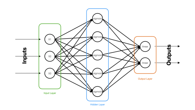
Figure 1: Schematic of the 3-layer Neural Network Regressor to be built. Input, hidden, and output layers are highlighted, and the relevant activation functions are written within each neuron.
The densely connected Neural Network illustrated in Figure 1 consists of 3 layers: a input, hidden, and output layer. The raw input predictor features (x1, x2, x3) are clamped to the input layer, that distributes these features to the hidden layer. The hidden layer consists of 5 neurons with sigmoid activation functions. The final output layer is made up of 2 neurons with linear activation functions. The choice of linear activations in the output layer is necessary for regression Neural Networks.
At a high level, the learning procedure will follow this sequence of steps:
- \text{for e} = 1..epochs:
- Do a Forward Pass
- Do a Backward Pass
- Update the model weights
For the sake of simplicity, the Backward Pass will make use of backpropagation with batch gradient descent. As such, we will only need to iterate through our training procedure for the number of epochs desired (as all the training data will be applied when updating the weights at each iteration).
To generate predictions we will need to do a single Forward Pass, with a trained model, on a set of input predictor features.
Implementation of a Multilayer Perceptron Regressor
We can now proceed to implement our Neural Network Regressor. As mentioned previously, if you’re interested in the technical details for how this algorithm is structured mathematically, please see my previous article on this subject.
To start let’s import all the packages required:
# imports
from typing import List, Tuple
import numpy as np
from sklearn.datasets import make_regression
from sklearn.model_selection import train_test_split
from sklearn.metrics import mean_squared_error, mean_absolute_error
import matplotlib.pyplot as plt
I will encapsulate the implementation within a single class, MLP352Regressor. Let’s now setup the initialiser and destructor functions:
class MLP352Regressor(object):
    """
    Class to encapsulate a Multilayer Perceptron / FeedForward Neural Network regressor
    """

    def __init__(self, lr: float=1e-2, epochs: int=100) -> None:
        """
        Initialiser function for a class instance

        Inputs:
            lr      -> learning rate
            epoches -> number of epoches to use during training
        """
        self.lr      = lr
        self.epochs  = epochs
        self.layers  = [3,5,2]
        self.weights = []
        self.biases  = []
        self.loss    = []

    def __del__(self) -> None:
        """
        Destructor function for a class instance
        """
        del self.lr
        del self.epochs
        del self.layers
        del self.weights
        del self.biases
        del self.loss
The loss I will use is the squared difference error. We can implement this along with it’s derivative with respect to the predictions \vec{y}^{pred}:
    def _loss(self, y_true: np.array, y_pred: np.array) -> np.array:
        """
        Function to compute squared-error loss per sample

        Inputs:
            y_true -> numpy array of true labels
            y_pred -> numpy array of prediction values
        Output:
            loss value
        """
        return 0.5*(y_true - y_pred)**2

    def _derivative_loss(self, y_true: np.array, y_pred: np.array) -> np.array:
        """
        Function to compute the derivative of the squared-error loss per sample

        Inputs:
            y_true -> numpy array of true labels
            y_pred -> numpy array of prediction values
        Output:
            loss value
        """
        return -(y_true - y_pred)
Both sigmoid and linear activation functions will be used in this class. Let’s define these, along with their derivatives \frac{df}{dz}:
    def _sigmoid(self, z: np.array) -> np.array:
        """
        Function to compute sigmoid activation function

        Input:
            z -> input dot product w*x + b
        Output:
            determined activation
        """
        return 1/(1+np.exp(-z))

    def _derivative_sigmoid(self, z: np.array) -> np.array:
        """
        Function to compute the derivative of the sigmoid activation function

        Input:
            z -> input dot product w*x + b
        Output:
            determined derivative of activation
        """
        return self._sigmoid(z)*(1 - self._sigmoid(z))

    def _linear(self, z: np.array) -> np.array:
        """
        Function to compute linear activation function

        Input:
            z -> input dot product w*x + b
        Output:
            determined activation
        """
        return z

    def _derivative_linear(self, z: np.array) -> np.array:
        """
        Function to compute the derivative of the linear activation function

        Input:
            z -> input dot product w*x + b
        Output:
            determined derivative of activation
        """
        return np.ones(z.shape)
We can now put together all the code needed for a single Forward Pass through the network:
    def _forward_pass(self, X: np.array) -> Tuple[List[np.array], List[np.array]]:
        """
        Function to perform forward pass through the network

        Input:
            X -> numpy array of input predictive features with assumed shape [number_features, number_samples]
        Output:
            list of activations & derivatives for each layer
        """
        # record from input layer
        input_to_layer = np.copy(X)
        activations    = [input_to_layer]
        derivatives    = [np.zeros(X.shape)]

        # hidden layer
        z_i = np.matmul(self.weights[0],input_to_layer) + self.biases[0]
        input_to_layer = self._sigmoid(z_i)
        activations.append(input_to_layer)
        derivatives.append(self._derivative_sigmoid(z_i))

        # output layer
        z_i = np.matmul(self.weights[1],input_to_layer) + self.biases[1]
        input_to_layer = self._linear(z_i)
        activations.append(input_to_layer)
        derivatives.append(self._derivative_linear(z_i))

        # return results
        return(activations, derivatives)
Similarly, the logic required for a single Backward Pass can also be placed in its own function:
    def _backward_pass(self,
                       activations: List[np.array],
                       derivatives: List[np.array],
                       y: np.array) -> Tuple[List[np.array], List[np.array]]:
        """
        Function to perform backward pass through the network

        Inputs:
            activations -> list of activations from each layer in the network
            derivatives -> list of derivatives from each layer in the network
            y           -> numpy array of target values
                           with assumed shape [output dimension, number_samples]
        Output:
            list of numpy arrays containing the derivates of the loss function wrt layer weights
        """
        # record loss
        self.loss.append((1/y.shape[1])*np.sum(self._loss(y, activations[-1])))

        # output layer
        dl_dy2 = self._derivative_loss(y, activations[2])
        dl_dz2 = np.multiply(dl_dy2, derivatives[2])
        dl_dw2 = (1/y.shape[1])*np.matmul(dl_dz2, activations[1].T)
        dl_db2 = (1/y.shape[1])*np.sum(dl_dz2, axis=1)

        # hidden layer
        dl_dy1 = np.matmul(self.weights[1].T, dl_dz2)
        dl_dz1 = np.multiply(dl_dy1, derivatives[1])
        dl_dw1 = (1/y.shape[1])*np.matmul(dl_dz1, activations[0].T)
        dl_db1 = (1/y.shape[1])*np.sum(dl_dz1, axis=1)

        # return derivatives
        return([dl_dw1, dl_dw2], [dl_db1, dl_db2])
Let’s write one last protected function to take care of updating the model weights and biases:
    def _update_weights(self, dl_dw: List[np.array], dl_db: List[np.array]) -> None:
        """
        Function to apply update rule to model weights

        Input:
            dl_dw -> list of numpy arrays containing loss derivatives wrt weights
        """
        self.weights[0] -= self.lr*dl_dw[0]
        self.weights[1] -= self.lr*dl_dw[1]
        self.biases[0]  -= self.lr*dl_db[0].reshape(-1,1)
        self.biases[1]  -= self.lr*dl_db[1].reshape(-1,1)
We now have all the protected member functions done for this class. Let’s now write two public functions that a developer can interact with, fit and predict:
    def fit(self, X: np.array, y: np.array) -> None:
        """
        Function to train a class instance

        Inputs:
            X -> numpy array of input predictive features with assumed shape [number_samples, number_features]
            y -> numpy array of target values with assumed shape [number_samples, output dimension]
        """
        # initialise the model parameters
        self.weights.clear()
        self.biases.clear()
        self.loss.clear()
        for idx in range(len(self.layers)-1):
            self.weights.append(np.random.randn(self.layers[idx+1], self.layers[idx]) * 0.1)
            self.biases.append(np.random.randn(self.layers[idx+1], 1) * 0.1)
        # loop through each epoch
        for _ in range(self.epochs):
            # do forward pass through the network
            activations, derivatives = self._forward_pass(X.T)
            # do backward pass through the network
            dl_dw, dl_db = self._backward_pass(activations, derivatives, y.T)
            # update weights
            self._update_weights(dl_dw, dl_db)

    def predict(self, X: np.array) -> np.array:
        """
        Function to produce predictions from a trained class instance

        Input:
            X -> numpy array of input predictive features with assumed shape [number_samples, number_features]
        Output:
            numpy array of model predictions
        """
        # do forward pass through the network
        activations, _ = self._forward_pass(X.T)
        # return predictions
        return activations[2].T
Create a Toy Dataset
Let’s produce a dataset by making use of scikit-learn’s make_regression, with 10000 samples, 3 predictive input features, and targets with a dimension of 2. Some minimal gaussian noise is also added:
# generate data
X, y = make_regression(n_samples=10000, n_features=3, n_targets=2, noise=1, random_state=42)
We can produce some box plots to get a sense of the distribution in these data:
plt.boxplot(X)
plt.title("Distribution of Input Predictive Features")
plt.xlabel("feature")
plt.ylabel("input unit")
plt.show()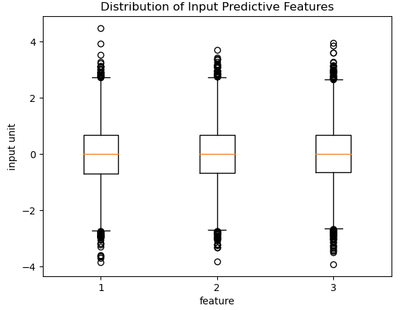
Figure 2: Distribution of input predictive features. All three features are approximately zero-centered, and range mostly between (-3,+3). Some outliers are present.
plt.boxplot(y)
plt.title("Distribution of Targets")
plt.xlabel("target")
plt.ylabel("output unit")
plt.show()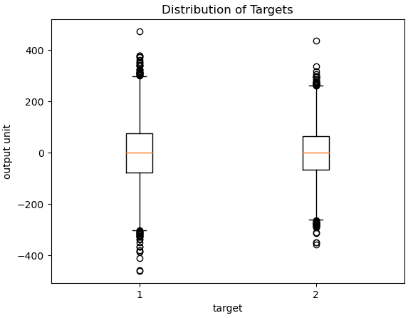
Figure 3: Distribution of output targets. The two features are approximately zero-centered, and range mostly between (-300,+300). Some outliers are present.
Finally, we can do a train-test split. We’ll allocate 80% of the data for training, and the remainder will be left for testing:
# perform train-test split
X_train, X_test, y_train, y_test = train_test_split(X, y, test_size=0.2, random_state=42)
Test our Multilayer Perceptron Regressor
We now have everything in place to test out our Neural Network! Let’s create an instance of our implemented class, and train it on the training data. I’ll use a learning rate of 0.01, and we’ll train for 1500 epochs:
# train the regressor
model = MLP352Regressor(lr=0.01, epochs=1500)
model.fit(X_train,y_train)
As a sanity check, let’s view the recorded loss as a function of epochs:
# plot the training loss
plt.plot(model.loss)
plt.title("Training Loss")
plt.xlabel("epochs")
plt.ylabel("loss")
plt.show()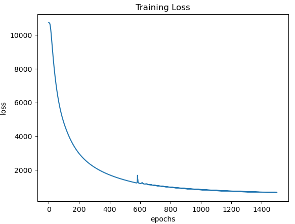
Figure 4: Training loss as a function of epochs.
Plotting the training loss shows a smooth decline in the loss value as each subsequent epoch is executed. This highlights that our training procedure is working as expected. Now let’s evaluate how well our regressor performs in making predictions:
# generate predictions
y_pred = model.predict(X_test)

# evaluate model performance
print(f"mse: {mean_squared_error(y_test, y_pred):.2f} and mae: {mean_absolute_error(y_test, y_pred):.2f}")
mse: 664.84 and mae: 16.53
y_testarray([[ 96.0652615 , 105.2753081 ],
[ 70.01592472, 169.33894413],
[ 136.81237065, 165.87554143],
...,
[ -76.98996266, -113.78059034],
[ 206.96193285, 256.91509498],
[ -39.808533 , -9.71756154]]) y_predarray([[ 97.76151633, 101.12347451],
[ 70.88374713, 99.54522216],
[ 136.31562322, 126.56560826],
...,
[ -85.5870685 , -100.21340972],
[ 169.65014163, 141.53248125],
[ -46.55959464, -9.32616964]]) Looking at these numbers, it’s evident that while most of the visible predictions are fairly reasonable, there are some cases where the deviation between prediction and truth is significant. This isn’t necessarily surprising, as Figure’s 2 & 3 do show the presence of outliers in both the input predictive features and targets. It is plausible that the presence of these outliers, in the training data, has degraded the overall performance of our regressor.
Final Remarks
In this post we have covered:
- The general architecture of a Multilayer Perceptron Regressor.
- How to implement a Multilayer Perceptron Regressor from scratch just using numpy.
- How to test our implementation to confirm that it works.
I hope you enjoyed this article, and gained some value from it. If you would like to take a closer look at the code presented here, please take a look at my GitHub. If you have any questions or suggestions, please feel free to add a comment below. Your input is greatly appreciated.
Related Posts
Hi I'm Michael Attard, a Data Scientist with a background in Astrophysics. I enjoy helping others on their journey to learn more about machine learning, and how it can be applied in industry.