Neural Network activation functions are used to control how artificial neurons respond to inputs. Seven of the most common, and popular, activation functions are covered in this post. They include the Sigmoid, Tanh, ReLU, Linear, Binary Threshold, Softmax, and Stochastic Binary functions. With the exception of the Linear activation, all of these functions introduce non-linearity into the Neural Network. This enables the model to learn highly complex relationships, that may be present in the data.
Table of Contents

7 Popular Types of Neural Network Activation Functions – image by Abi Plata
What are Neural Network Activation Functions?
Neural Networks are a family of machine learning algorithms that seek to emulate how biological brains work. Like their biological counterparts, Neural Networks are made up of a series of interconnected neurons. Information flows into the neuron, is assessed internally, and then a response is sent out. Biological neurons receive information through a set of dendrites, which branch out from the cell body. The received information is assessed internally within the cell, and then a response is sent out via the axon to other neurons. This anatomy is depicted in Figure 1 below:

Figure 1: Anatomy of a biological neuron. The cell is connected to other neurons via it’s dendrites (inputs) and axon (output). Image by Clker-Free-Vector-Images from Pixabay.
Within Neural Networks, artificial neurons mimic this structure. Information is received from a set of inputs defined by a vector \vec{x}. The input data is processed, and an output response y is sent out to other neurons in the network, or as a final output from the entire network. This structure is outlined in Figure 2 below:
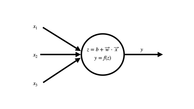
Figure 2: Structure of an artificial neuron. In this example, the neuron has 3 inputs x_1, x_2, and x_3. The output from the neuron is represented by y.
In this particular case, we can see that \vec{x} = \begin{bmatrix} x_1 \\ x_2 \\ x_3 \end{bmatrix} . Note that in general, there can be an arbitrary number of inputs. Within the neuron, the quantity z is computed by taking the dot product of \vec{x} with a vector of input weights \vec{w}, and adding the bias term b. The output y is finally obtained by applying the activation function of the neuron f to z.
Normally f is a non-linear function. Without this non-linearity, the most complex Neural Network would only be able to do linear modelling. It is the combination of many artificial neurons, each with their own non-linear f, that give Neural Networks such enormous potential to find complex relationships in the data.
Types of Neural Network Activation Functions
Before jumping into the descriptions for each activation function, note that the examples make use of numpy and matplotlib:
# imports
from typing import Tuple
import numpy as np
import matplotlib.pyplot as plt
Sigmoid Activation Function
Here the activation behaves according to the sigmoid, or logistic, function:
y = \frac{1}{1+e^{-z}}
This function is smooth and continuous, with a bounded output between [0,1]. The derivatives of this function are easy to compute, and this helps when training a Neural Network. Because of this properly, sigmoid activation functions were once the most popular choice for use within Neural Networks. That title has since been taken by the tanh & ReLU activation functions, due to their superior performance. For binary classification problems, the sigmoid activation function is still used in the output layer of Neural Networks.
Let’s implement the sigmoid function is Python, and then visualise its form:
def sigmoid(z : np.array) -> np.array:
    """
    Function to execute the sigmoid activation

    Inputs:
        z : input dot product w*x + b
    Output:
        y : determined activation
    """
    return 1/(1+np.exp(-z))

z = np.linspace(-5,5,num=100)
y = sigmoid(z)

plt.plot(z,y)
plt.xlabel('z')
plt.ylabel('y')
plt.title('Sigmoid Activation Function')
plt.show()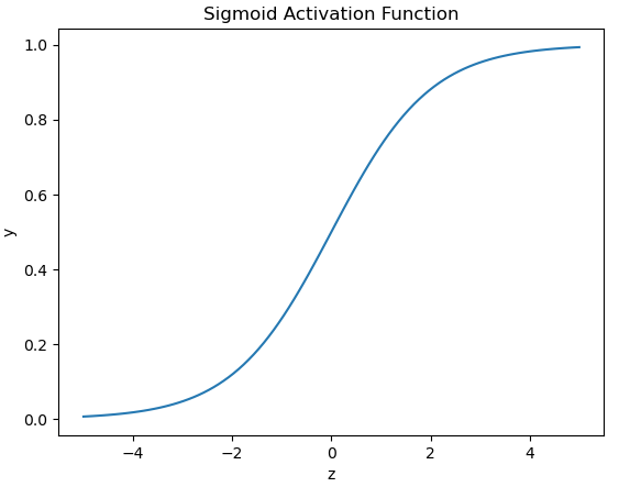
Tanh Activation Function
Here the activation behaves according to the hyperbolic tan (tanh) function:
y = \frac{e^z – e^{-z}}{e^z+e^{-z}}
This function is also smooth and continuous, like the sigmoid function. However, the bounds for the output are between [-1,1]. In practice, these activation functions almost always perform better than the sigmoid function, due to the mean of their output being 0 (which can help in the training of subsequent layers in the Neural Network).
Let’s implement the tanh function is Python, and then visualise its form:
def tanh(z : np.array) -> np.array:
    """
    Function to execute the tanh activation

    Inputs:
        z : input dot product w*x + b
    Output:
        y : determined activation
    """
    return (np.exp(z) - np.exp(-z))/(np.exp(z)+np.exp(-z))

z = np.linspace(-5,5,num=100)
y = tanh(z)

plt.plot(z,y)
plt.xlabel('z')
plt.ylabel('y')
plt.title('Tanh Activation Function')
plt.show()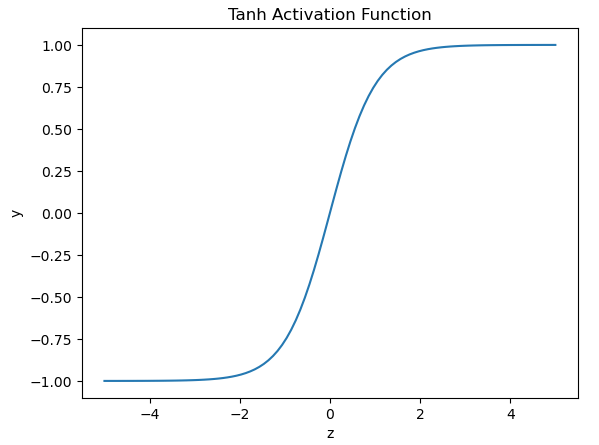
Linear Activation Function
This is the sole activation covered here that is linear. It yields a continuous output according to y = z. Note that in this case f is the identity function, and therefore we do not need to explicitly implement it in code for our example below. These activations are typically used in the output layer of Neural Networks modelling regression problems.
Let’s visualise the linear activation:
z = np.linspace(-4,4,num=100)

plt.plot(z,z)
plt.xlabel('z')
plt.ylabel('y')
plt.title('Linear Activation Function')
plt.show()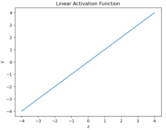
ReLU Activation Function
The Rectified Linear Unit (ReLU) activation behaves according to:
y = \begin{cases} z & z \ge 0 \\ 0 & z \lt 0 \end{cases}
This piecewise function behaves like the linear activation for positive z values, and remains fixed at 0 otherwise. The main advantage of this activation over the sigmoid or tanh functions is that it retains large derivatives for increasing values of z. Since the sigmoid & tanh functions are both asymtotic, their derivatives approach 0 for increasing large values of |z|. In practice this has the effect of slowing down training. The ability of ReLU activations to speed up training has made them a very popular choice for machine learning practitioners.
Let’s implement the ReLU function is Python, and then visualise its form:
def relu(z : np.array) -> np.array:
    """
    Function to execute the ReLU activation

    Inputs:
        z : input dot product w*x + b
    Output:
        y : determined activation
    """
    return np.where(z>=0,z,0)

z = np.linspace(-5,5,num=100)
y = relu(z)

plt.plot(z,y)
plt.xlabel('z')
plt.ylabel('y')
plt.title('ReLU Activation Function')
plt.show()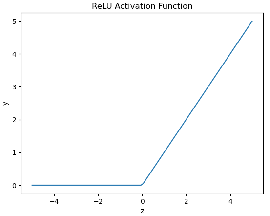
Binary Threshold Activation Function
This activation is a Heaviside step function of z. It has the following mathematical form:
These functions are most notably used in Perceptrons. They are unsuitable for Neural Networks that make use of backpropagation, as the gradient is zero or undefined.
Let’s implement the binary threshold function is Python, and then visualise its form:
def binary(z : np.array) -> np.array:
    """
    Function to execute the binary threshold activation

    Inputs:
        z : input dot product w*x + b
    Output:
        y : determined activation
    """
    return np.round(z >= 0)

z = np.linspace(-4,4,num=100)
y = binary(z)

plt.plot(z,y)
plt.xlabel('z')
plt.ylabel('y')
plt.title('Binary Threshold Activation Function')
plt.show()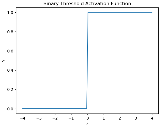
Softmax Activation Function
The Softmax activation is used strictly in the output layer of Neural Networks performing classification. The output from a single softmax neuron y_i follows the form:
y_i = \frac{e^{z_i}}{\sum_j^J e^{z_j}}
where z_i is the i^{th} element in z. This function yields a probability distribution over all J output classes. As such, the output y_i is bounded by (0,1). Softmax is a smooth approximation to the Argmax function, where the later produces the index of the maximum value within z. Argmax is unsuitable for direct use in Neural Networks, since this will only provide 0 or undefined gradients for backpropagation.
Let’s implement the softmax function is Python, and then visualise its form:
def softmax(z : np.array) -> np.array:
    """
    Function to execute the softmax activation

    Inputs:
        z : input dot product w*x + b
    Output:
        y : determined activation
    """
    return np.exp(z)/np.sum(np.exp(z))

z = np.linspace(-5,5,num=100)
y = softmax(z)

plt.plot(z,y)
plt.xlabel('z')
plt.ylabel('y')
plt.title('Softmax Activation Function')
plt.show()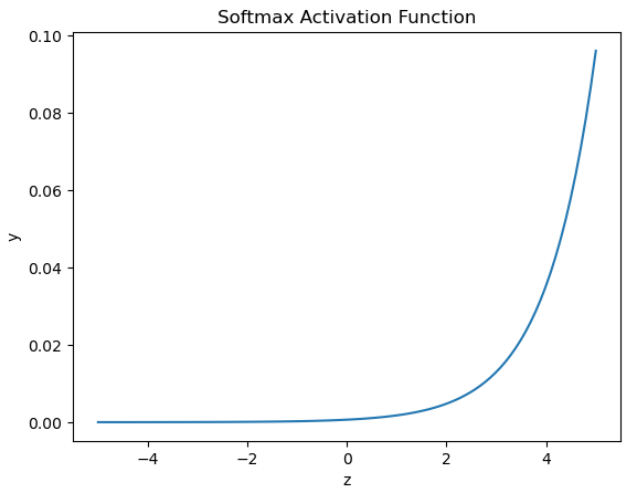
We can also verify the probabilistic nature of the output from the softmax function, through a simple 3-class example:
# example of probablistic output
z = np.array([4.3, 1.5, -10.3])
y = softmax(z)
y
array([9.42675419e-01, 5.73241512e-02, 4.30192413e-07])
np.sum(y)1.0
The output values are all lie between (0,1) and sum to 1.0. In addition, the order of the elements in z is preserved in the output: i.e. the largest probability (\approx0.94) is assigned to the largest element z_1 = 4.3. Clearly the output from the softmax function can be interpreted as probabilities.
Stochastic Binary Activation Function
These neurons behave in a probabilistic way, with their outputs being governed by a probability distribution. This distribution is given by the sigmoid function (which we have seen before with the Sigmoid Activation Function):
p(s=1) = \frac{1}{1+e^{-z}}
However, the neuron does not output the value of this function. Instead p(s=1) is the probability of a state 1 being returned, given the input. Conversely, 1 – p(s=1) is the probability of obtaining a state 0.
These neurons are used in Energy-Based models, such as Restricted Boltzmann Machines (RBMs) or Deep Belief Networks (DBNs).
We can now implement the stochastic binary activation function in Python. With this implementation, we can plot the probability distribution p(s=1), and the actual output:
def stochastic(z : np.array) -> Tuple[np.array,np.array]:
    """
    Function to execute the stochastic binary activation

    Inputs:
        z : input dot product w*x + b
    Output:
        (y,p_s) : determined activation, and probability of returning a 1
    """
    p_s = 1/(1+np.exp(-z))
    return np.array([np.random.choice([1,0],p=[p,1-p]) for p in p_s]),p_s

z   = np.linspace(-5,5,num=100)
y,p = stochastic(z)

plt.plot(z,p)
plt.xlabel('z')
plt.ylabel('p')
plt.title('Probability of s=1')
plt.show()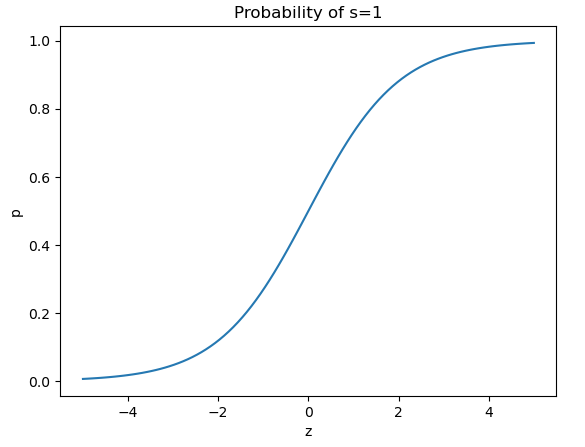
plt.plot(z,y)
plt.xlabel('z')
plt.ylabel('y')
plt.title('Stochastic Binary Activation Function')
plt.show()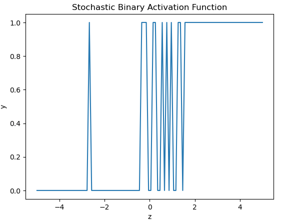
We can see the output from the activation function tends to 0 for increasingly large negative values of z. Conversely, the output tends to 1 for increasingly large positive values of z. In the vicinity of z \approx 0, the output oscillates wildly between 0 and 1. This makes senes in terms of the probability distribution that governs the state of y.
Final Remarks
This article outlined 7 of the most popular Neural Network activation functions. My intention here was to provide motivation for you to learn these functions, and outline simple descriptions for each of them. I hope that you enjoyed this content, and gained some value from it. If you have any questions or comments, please leave them below!
Related Posts
Hi I'm Michael Attard, a Data Scientist with a background in Astrophysics. I enjoy helping others on their journey to learn more about machine learning, and how it can be applied in industry.
