This article will cover an implementation of the Perceptron algorithm from scratch in Python. First we will talk about the motivation behind the Perceptron, along with a brief history of its development. Next, the underlying assumptions and considerations will be covered, before outlining the algorithm itself. Finally, we will implement the algorithm into Python code, and test its performance on two different datasets.
Table of Contents

Implement the Perceptron Algorithm from Scratch in Python – image by author
Motivation for the Perceptron
The Perceptron arose out of the desire to model the behaviour of individual biological neurons. This algorithm is the simplest and oldest type of neural network, with its roots dating back to the 1940’s. It is intended for use in classification problems.
The foundations of the Perceptron algorithm were made by Warren McCulloch and Walter Pitts in their 1943 paper “A Logical Calculus of Ideas Immanent in Nervous Activity“. Their work conceived the idea of using a binary threshold activation function to make logical decisions, based upon the input received. Frank Rosenblatt expanded upon these ideas, to develop the first Perceptron as we would recognise it today. His work, published in the 1962 book “Principles of Neurodynamics“, greatly popularised this algorithm at the time.
Marvin Minsky and Seymour Papert, in their 1969 book “Perceptrons: An Introduction to Computational Geometry“, illustrated the limitations to what Perceptrons could actually do. These include the dependance on linear separability, as well as the inability for these algorithms to learn patterns transformed by a wrap-around function. These issues can be resolved with careful feature engineering, but this was not a satisfactory solution to these problems.
The eventual development of multi-layered neural networks, where various hidden layers serve to automatically learn the features required, resolved the problems raised by Minsky and Papert. This achievement kick-started the rapid development of neural networks from the 1980’s to the present day.
Assumptions and Considerations
Some points to keep in mind when thinking about this algorithm:
- Perceptrons are highly dependent on the features that are fed into it. Most importantly, the classes within the data need to be linearly separable. Therefore, attention must be given to the feature engineering prior to training the model.
- Perceptrons are designed to work on supervised classification problems.
- The algorithm is relatively simple, and easy to implement. As such, training proceeds quickly, and the algorithm scales quite well to very large datasets.
The Perceptron Algorithm
For the sake of simplicity, I will only consider the binary classification problem with labels [0,1]. We can get a feel for how this algorithm is structured, through a simple visualisation:
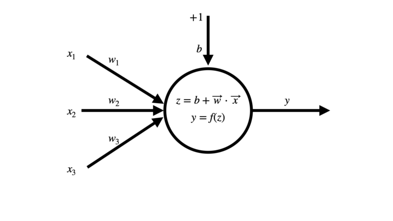
Figure 1: Illustration of a Perceptron consisting of 3 input features. The input features \vec{x} = [x_1, x_2, x_3] are weighted by \vec{w} = [w_1, w_2, w_3]. A bias term of +1 is also present, and weighted by b. An activation function f is applied to the dot product of the inputs and weights, to yield an output y.
The figure above outlines the basic flow through the model. A set of hand-written features \vec{x} are provided as input, and are weighted by a vector \vec{w} with an equal number of elements. A bias term can also be added, that consists of an input fixed at +1 with weight b. In this way, the bias can be treated exactly the same as the other inputs. The dot product z of the inputs and weights is computed, and subsequently an activation function f is applied to yield a prediction y. Note that the number of inputs to the model can be an arbitrary integer.
Our problem then becomes how to determine \vec{w}? This will need to be calculated using the available training data of N samples:
\bold{X} = \begin{bmatrix} \vec{x}_1 \\ \vec{x}_2 \\ … \\ \vec{x}_N \end{bmatrix}
\vec{y} = [y_1, y_2, … y_N]
Note that each \vec{x}_i is a row vector in matrix \bold{X}. The algorithm for accomplishing this task is as follows:
- Iterate through each sample i = 1..N:
- Compute z_i = b + \vec{w} \cdot \vec{x}_i
- Compute y^{\text{pred}}_i = f(z_i)
- Compare the prediction with the true class label y^{\text{true}}_i:
- If the prediction matches the true class label, no updates
- If y^{\text{pred}}_i = 0, when it should be a 1, update the weights with \vec{w} \Longleftarrow \vec{w} + \vec{x}
- If y^{\text{pred}}_i = 1, when it should be a 0, update the weights with \vec{w} \Longleftarrow \vec{w} – \vec{x}
Furthermore, the algorithm above can be repeated a number of times as well. Each cycle through the training data represents an epoch in our training procedure.
Once \vec{w} is known, we can then use our trained model to make predictions unseen samples. This will happen by cycling through each sample, and executing steps 1. and 2. described above.
Build and Test a Perceptron in Python
We’ll now seek to implement the algorithm described in the previous section. Once we’re done with this, we will test out our custom implementation on 2 toy datasets. In addition, we’ll compare the performance of our implementation with the Perceptron available from scikit-learn.
To start, let’s import all the packages required for our implementation and testing:
# imports
import numpy as np
from typing import Dict, List
import matplotlib.pyplot as plt
from sklearn.model_selection import train_test_split
from sklearn.datasets import make_blobs, make_circles
from sklearn.metrics import accuracy_score, \
                            precision_score, \
                            recall_score, \
                            f1_score
Implement a Perceptron from Scratch
Our Perceptron implementation will be encapsulated within a single Python class. This implementation, in its entirely, is presented below:
class Perceptron(object):
    """
    Class to encapsulate the Perceptron algorithm
    """

    def __init__(self, lr: float=1e-2, max_epochs: int=100, tol: float=1e-3, verbose: bool=False) -> None:
        """
        Initialiser function for a class instance

        Inputs:
            lr         -> learning rate; factor to determine how much weights are updated at each pass
            max_epochs -> maximum number of epochs the algorithm is allowed to run before stopping
            tol        -> tolerance to stop training procedure
            verbose    -> boolean to determine if extra information is printed out
        """
        if lr <= 0:
            raise ValueError(f'Input argument lr must be a positive number, got: {lr}')
        if max_epochs <= 0:
            raise ValueError(f'Input argument max_epochs must be a positive integer, got: {max_epochs}')
        if tol <= 0:
            raise ValueError(f'Input argument tol must be a positive number, got: {tol}')
        self.lr            = lr
        self.epochs        = max_epochs
        self.tol           = tol
        self.w             = np.array([])
        self.verbose       = verbose
        self.training_loss = []
        if self.verbose:
            print(f'Creating instance with parameters: lr = {self.lr}, max_epochs = {self.epochs}, and tol = {self.tol}')

    def __del__(self) -> None:
        """
        Destructor function for class instance
        """
        del self.lr
        del self.epochs
        del self.tol
        del self.w
        del self.verbose
        del self.training_loss

    def fit(self, X : np.array, y : np.array) -> None:
        """
        Training function for the class. Runs the training algorithm for the number of epochs set in the initialiser

        Inputs:
            X -> numpy array of input features of assumed shape [number_samples, number_features]
            y -> numpy array of binary labels of assumed shape [number_samples]
        """
        # add column for bias
        X = np.insert(X, 0, 1, axis=1)
        # initialise the weights
        self.w = np.zeros(X.shape[1])
        # initialise loss
        loss = 1e8

        # loop through the training procedure for the specified number of epochs
        for e in range(self.epochs):

            epoch_loss = 0

            # loop through each training sample
            for x_i,y_i in zip(X,y):

                # compute activation
                z  = np.dot(x_i,self.w)
                yp = np.round(z >= 0)
                # update weights
                self.w += self.lr*(y_i-yp)*x_i
                # record the loss
                epoch_loss += np.abs(y_i-yp)

            # check for early stopping
            new_loss = (1/X.shape[0])*epoch_loss
            if (loss < (new_loss - self.tol)) or (new_loss < self.tol):
                if self.verbose:
                    print(f'Early stopping training procedure at Epoch: {e}, Loss: {new_loss}')
                break
            else:
                loss = new_loss
                self.training_loss.append(loss)
                if self.verbose:
                    print(f'Epoch: {e}, Loss: {loss}')

    def predict(self, X : np.array) -> np.array:
        """
        Predict function for the class. Assigns class label based on learned weights and the binary threshold
        activation

        Input:
            X -> numpy array of input features of assumed shape [number_samples, number_features]
        Output:
            numpy array indicating class assignment per sample with shape: [number_samples,]
        """
        if self.w.size == 0:
            raise Exception("It doesn't look like you have trained this model yet!")
        # add column for bias
        X = np.insert(X, 0, 1, axis=1)
        # compute dot products for all training samples
        z = np.einsum('ij,j->i', X, self.w)
        # pass through activation function, and return
        yp = np.round(z >= 0)
        return yp

    def get_weights(self) -> np.array:
        """
        Function to return model weights

        Output:
            numpy array containing the model weights
        """
        return self.w

    def get_training_loss(self) -> List:
        """
        Function to return training loss

        Output:
            list containing the training loss, one entry per epoch
        """
        return self.training_loss

    def get_params(self, deep : bool = False) -> Dict:
        """
        Public function to return model parameters
        Inputs:
            deep -> boolean input parameter
        Outputs:
            Dict -> dictionary of stored class input parameters
        """
        return {'lr':self.lr,
                'max_epochs':self.epochs,
                'tol':self.tol,
'verbose':self.verbose}- __init__(self, lr, max_epochs, tol, verbose) : this is the initialiser function for each class instance. The learning rate (lr) defines how large the updates to the weights will be with each training iteration. The number of times the training procedure will be repeated (i.e. epochs) is defined by the parameter max_epochs. Early stopping of the training procedure is controlled by tol, which sets a threshold for our loss function. Finally, verbose controls whether extra information is printed out at runtime. All internal class-wide variables are initialised in this function.
- __del__(self) : destructor function for each class instance. Releases allocated resources once the instance is deleted.
- fit(self, X, y): public function to execute the training procedure outlined in the previous section of this post, for training data X and y. Three things to note:
- I am making use of the binary threshold activation function.
- The training loss function is: loss = \sum_i^N |y^{\text{true}}_i – y^{\text{pred}}_i|.
- I assume the input features X have not been treated for the bias. As such, within this implementation I add a column of ones to this matrix.
- predict(self, X) : public function used to generated predictions from a trained model instance. Predictions are based off of the array of input feature samples X. Like with the fit function, here I assume a column of ones needs to be added to X to account for the bias.
- get_weights(self) : public function used to return the model weights.
- get_training_loss(self) : public function used to return the training loss.
- get_params(self, deep) : public function used to return the model hyperparameters. This function is necessary if we want to make use of any scikit-learn functionality with our class instances.
Dataset Example #1
Let’s start by creating our first toy dataset, with scikit-learn’s make_blobs function:
# make a dataset
X,y = make_blobs(n_samples=1000, centers=2, n_features=2, cluster_std=0.5, random_state=0)

# visualise the data
fig, ax = plt.subplots(figsize=(10,8))
sc      = ax.scatter(X[:,0],X[:,1],c=y)
plt.xlabel('x1')
plt.ylabel('x2')
plt.title('Distribution of Data with True Class Labels')
ax.legend(*sc.legend_elements(), title='classes')
plt.show()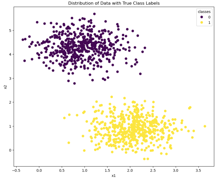
Figure 2: toy dataset #1.
We have produced a dataset consisting of 1000 samples, two predictor features, and 2 class labels. Looking at figure 2, it is evident that the two classes are linearly separable.
Now let’s do a train-test split of our data, declare an instance of our Perceptron, and train it:
# do train test split
X_train, X_test, y_train, y_test = train_test_split(X, y, test_size=0.2, random_state=42)

# declare an instance of our Perceptron class
model1 = Perceptron(lr=0.1, verbose=True)
Creating instance with parameters: lr = 0.1, max_epochs = 100, and tol = 0.001
# fit the model on our training data
model1.fit(X_train,y_train)
Epoch: 0, Loss: 0.01375 Epoch: 1, Loss: 0.01375 Epoch: 2, Loss: 0.00625 Epoch: 3, Loss: 0.00625 Epoch: 4, Loss: 0.00625 Epoch: 5, Loss: 0.00375 Epoch: 6, Loss: 0.0025 Early stopping training procedure at Epoch: 7, Loss: 0.0
Twenty percent of the data has been held-out for testing. I have set the learning rate for our Perceptron to 0.1, and I’ve also requested the verbose mode on. Having the model run in verbose mode means the training loss is printed out, and we can see that early stopping is reached at epoch 7 with 0.0 loss.
Now let’s use the trained model to generate predictions on the test set. Next, we can see how well our classifier has performed using the accuracy, precision, recall, and F1 scores:
# generate predictions on the test set
y_pred = model1.predict(X_test)

# how accurate are the predictions?
acc = accuracy_score(y_test,y_pred)
pre = precision_score(y_test,y_pred,average='weighted')
rec = recall_score(y_test,y_pred,average='weighted')
f1  = f1_score(y_test,y_pred,average='weighted')
print(f'Accuracy score: {acc:.4f}')
print(f'Precision score: {pre:.4f}')
print(f'Recall score: {rec:.4f}')
print(f'F1 score: {f1:.4f}')
Accuracy score: 1.0000 Precision score: 1.0000 Recall score: 1.0000 F1 score: 1.0000
We have a perfect score! This shouldn’t be too surprising: we already know that the dataset is linearly separable. Also, the Perceptron learned to differentiate between the two classes in the training set perfectly.
Now let’s repeat this analysis, but make use of the Perceptron available from scikit-learn:
# check out what we get from the scikit-learn Perceptron?
from sklearn.linear_model import Perceptron as sklearn_Perceptron

model2 = sklearn_Perceptron(random_state=42)
model2.fit(X_train,y_train)
y_pred = model2.predict(X_test)

acc = accuracy_score(y_test,y_pred)
pre = precision_score(y_test,y_pred,average='weighted')
rec = recall_score(y_test,y_pred,average='weighted')
f1  = f1_score(y_test,y_pred,average='weighted')
print(f'Accuracy score: {acc:.4f}')
print(f'Precision score: {pre:.4f}')
print(f'Recall score: {rec:.4f}')
print(f'F1 score: {f1:.4f}')
Accuracy score: 1.0000 Precision score: 1.0000 Recall score: 1.0000 F1 score: 1.0000
Again we have a perfect score, and again this shouldn’t be surprising. So far the behaviour of our custom implementation matches that of the scikit-learn model.
Dataset Example #2
We can now create a second toy dataset. But this time we will make use of scikit-learn’s make_circles function:
# make a dataset
X,y = make_circles(n_samples=1000, noise=0.03, random_state=0)

# visualise the data
fig, ax = plt.subplots(figsize=(10,8))
sc      = ax.scatter(X[:,0],X[:,1],c=y)
plt.xlabel('x1')
plt.ylabel('x2')
plt.title('Distribution of Data with True Class Labels')
ax.legend(*sc.legend_elements(), title='classes')
plt.show()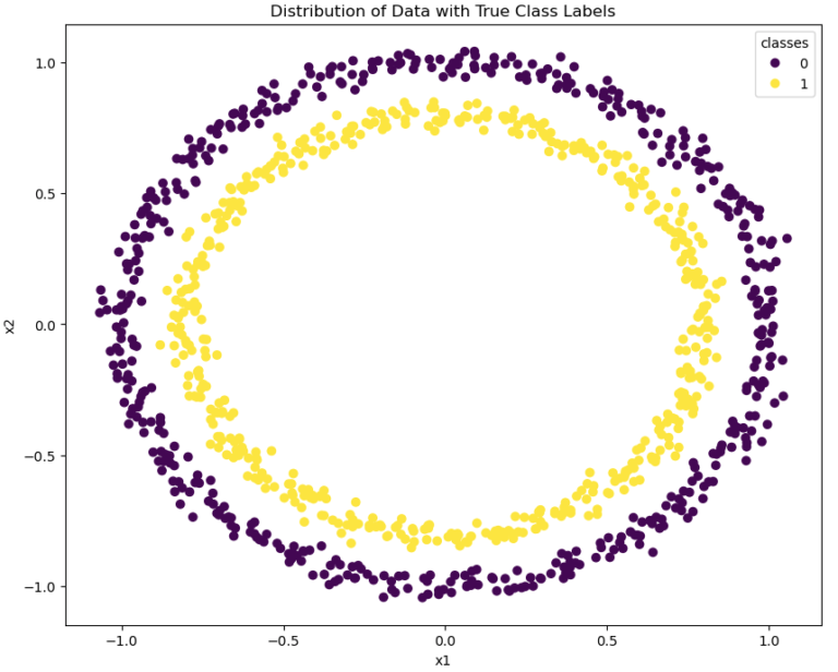
Figure 3: toy dataset #2.
Unlike the previous dataset, here the two classes are situated in concentric rings. As such, these classes are not linearly separable. Now how well does our Perceptron perform?
# do train test split
X_train, X_test, y_train, y_test = train_test_split(X, y, test_size=0.2, random_state=42)

# fit the model on our training data
model1.fit(X_train,y_train)
Epoch: 0, Loss: 0.48875 Early stopping training procedure at Epoch: 1, Loss: 0.5025000000000001
# generate predictions on the test set
y_pred = model1.predict(X_test)

# how accurate are the predictions?
acc = accuracy_score(y_test,y_pred)
pre = precision_score(y_test,y_pred,average='weighted')
rec = recall_score(y_test,y_pred,average='weighted')
f1  = f1_score(y_test,y_pred,average='weighted')
print(f'Accuracy score: {acc:.4f}')
print(f'Precision score: {pre:.4f}')
print(f'Recall score: {rec:.4f}')
print(f'F1 score: {f1:.4f}')
Accuracy score: 0.4700 Precision score: 0.2209 Recall score: 0.4700 F1 score: 0.3005
It is evident that the classifier has not functioned well on these data. Our error metrics highlight the poor performance of the trained Perceptron. Furthermore, the training procedure stopped early as the loss increased after 1 epoch.
Can we get anything better with the scikit-learn implementation?
# fit the model on our training data
model2.fit(X_train,y_train)

# generate predictions on the test set
y_pred = model2.predict(X_test)

# how accurate are the predictions?
acc = accuracy_score(y_test,y_pred)
pre = precision_score(y_test,y_pred,average='weighted')
rec = recall_score(y_test,y_pred,average='weighted')
f1  = f1_score(y_test,y_pred,average='weighted')
print(f'Accuracy score: {acc:.4f}')
print(f'Precision score: {pre:.4f}')
print(f'Recall score: {rec:.4f}')
print(f'F1 score: {f1:.4f}')
Accuracy score: 0.5450 Precision score: 0.5471 Recall score: 0.5450 F1 score: 0.5454
Here too the results are poor, although the scikit-learn model does yield some-what better results.
What we need is to transform the input features for this dataset. This transformation must be done in such a way that the two classes become linearly separable. We can achieve this by converting these data to polar coordinates:
# convert features to polar coordinates
radius = np.sqrt(X[:,0]**2+X[:,1]**2)
theta  = np.arctan2(X[:,1],X[:,0])
X_pol  = np.concatenate((radius.reshape(-1,1),theta.reshape(-1,1)),axis=1)

# visualise the data
fig, ax = plt.subplots(figsize=(10,8))
sc      = ax.scatter(X_pol[:,0],X_pol[:,1],c=y)
plt.xlabel('radius')
plt.ylabel('theta')
plt.title('Distribution of Data with True Class Labels')
ax.legend(*sc.legend_elements(), title='classes')
plt.show()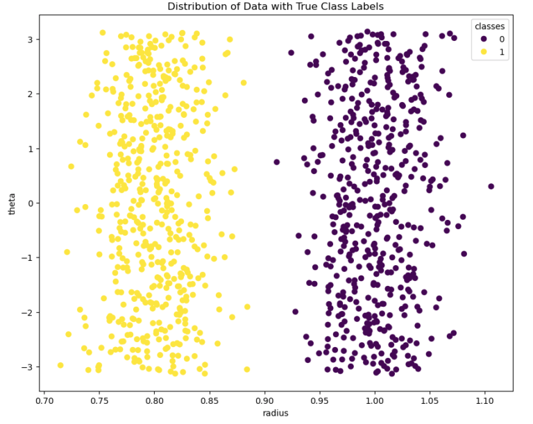
Figure 4: toy dataset #2, transformed into polar coordinates.
With our transformed features, let’s now repeat our analysis to see how the Perceptron models fair:
# do train test split
X_train, X_test, y_train, y_test = train_test_split(X_pol, y, test_size=0.2, random_state=42)

# fit the model on our training data
model1.fit(X_train,y_train)
Epoch: 0, Loss: 0.195 Early stopping training procedure at Epoch: 1, Loss: 0.0
# generate predictions on the test set
y_pred = model1.predict(X_test)

# how accurate are the predictions?
acc = accuracy_score(y_test,y_pred)
pre = precision_score(y_test,y_pred,average='weighted')
rec = recall_score(y_test,y_pred,average='weighted')
f1  = f1_score(y_test,y_pred,average='weighted')
print(f'Accuracy score: {acc:.4f}')
print(f'Precision score: {pre:.4f}')
print(f'Recall score: {rec:.4f}')
print(f'F1 score: {f1:.4f}')
Accuracy score: 1.0000 Precision score: 1.0000 Recall score: 1.0000 F1 score: 1.0000
Our custom implementation now yields a perfect score again! How does the scikit-learn model perform on these data?
# fit the model on our training data
model2.fit(X_train,y_train)

# generate predictions on the test set
y_pred = model2.predict(X_test)

# how accurate are the predictions?
acc = accuracy_score(y_test,y_pred)
pre = precision_score(y_test,y_pred,average='weighted')
rec = recall_score(y_test,y_pred,average='weighted')
f1  = f1_score(y_test,y_pred,average='weighted')
print(f'Accuracy score: {acc:.4f}')
print(f'Precision score: {pre:.4f}')
print(f'Recall score: {rec:.4f}')
print(f'F1 score: {f1:.4f}')
Accuracy score: 0.9950 Precision score: 0.9951 Recall score: 0.9950 F1 score: 0.9950
The scikit-learn model also does very well, however our custom implementation does better on these data by a small margin.
This highlights an important fact about Perceptrons: they are highly dependant on the hand-written input features. They cannot learn these on their own! Therefore, an essential step to make use of Perceptrons is to first perform a feature engineering stage prior to training. This stage aims at making the input features as linearly separable as possible, so as to give the model the best chance at optimal performance.
Final Remarks
In this article you have learned:
- What the Perceptron algorithm is, and when it was developed.
- The assumptions and considerations that need to be kept in mind when using the Perceptron algorithm.
- How to implement the Perceptron Algorithm from scratch in Python.
- How our custom implementation compares against the Perceptron available from scikit-learn.
I hope you enjoyed this article, and gained some value from it. If you would like to take a closer look at the code presented here, please take a look at my GitHub. If you have any questions or suggestions, please feel free to add a comment below. Your input is greatly appreciated.
Related Posts
Hi I'm Michael Attard, a Data Scientist with a background in Astrophysics. I enjoy helping others on their journey to learn more about machine learning, and how it can be applied in industry.