Neural Networks are complex machine learning models, that are structured in a way inspired by biological brains. The majority of supervised Neural Networks learn by making repeated passes through the training data. On each pass, data propagates forward through the network, to generate predictions. These predictions are then used to calculate a loss against the set of true labels. The effects of this loss are then passed backward through the network, by making use of the Backpropagation algorithm. The results of this backward pass can then be used to update the weights of the model, in such a way to minimise the loss.
Table of Contents

How Neural Networks Learn, with 1 Complete Example – image by author
Scope of the Article
There are a myriad of different types of Neural Network architectures, and various ways of learning. Covering them all is beyond the scope of this post. Instead, here I will focus on a common setup you will likely encounter for a regression problem. This includes the following attributes:
- Is a supervised problem (training labels are available, and we seek to build a model to make predictions)
- Hidden layers are included in the architecture (see Figure 1)
- Training procedure makes use of backpropagation
The generic type of network architecture, that has these attributes, is illustrated in Figure 1.
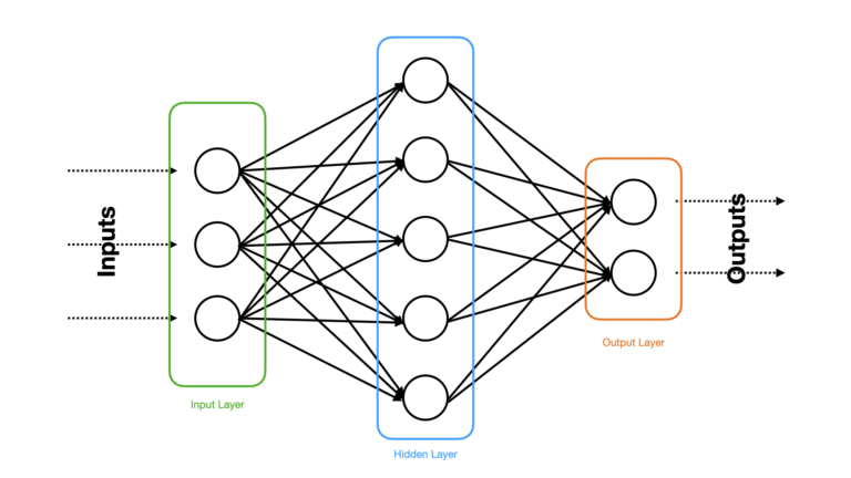
Figure 1: A simple example of a Feed Forward Neural Network. Circles indicate neurons, and arrows indicate weighted connections between neurons of different layers. Dashed arrows show inputs to, and outputs from, the model. Different layers have been named and highlighted.
The example in Figure 1 has only a single hidden layer, and a relatively small number of neurons per layer. This serves as a good illustration for the type of network I will be talking about in this article. Keep in mind that many state-of-the-art Neural Networks are considerably more complex than this.
Definition of Terms
Before diving into the details of the learning procedure, I would like to define 3 key terms. We will be using them throughout the remainder of the article:
- Epoch: a single pass through the entire training dataset
- Iteration: a single update to the weights in the model
- Batch: the number of data samples grouped together for a single iteration. This effectively describes way we partition the training data
To better understand how these 3 terms relate to one another, let’s consider the example in Figure 2:
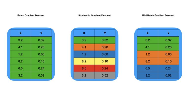
Figure 2: Example of partitioning the same training data under 3 different scenarios. Rows are grouped together has indicated by colour.
We can work through the example in Figure 2 left-to-right. First with the left-most image, we can see a simple dataset consisting of two columns, X and Y, with 6 rows. All the rows are grouped together, as indicted by the colour (green). In this case, all the data is used each time we update the weights of the model. Therefore, we have 1 batch (the whole dataset), and for each epoch there will be 1 iteration. This approach makes use of the optimisation procedure called Batch Gradient Descent.
Turning to the middle image, we see the same data as before, but with each row having a distinct colour. In this example, we update the weights for every sample in the data. Therefore, we have 6 “batches”, although no data is actually grouped together. For each epoch, there will be 6 iterations. This approach makes use of the optimisation procedure called Stochastic Gradient Descent.
Lastly, the image on the right again has the same data as the previous two examples. But we can see 3 groups of rows, as indicated by colour. Here we update the weights 3 times for a single pass through the data. As such, we have 3 batches, and for each epoch, there will be 3 iterations. The approach makes use of the optimisation procedure called Mini Batch Gradient Descent.
Components of the Learning Procedure
There are 2 key stages to training a Neural Network: a Forward Pass and Backward Pass through the network. Let’s describe these two in some more detail below.
Forward Pass
The Forward Pass through the network involves applying the predictive data features at the input layer, cascading the activations of the neurons through each successive layer, and producing output. This flow is illustrated in Figure 3 below:
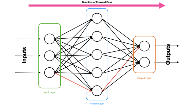
Figure 3: Propagation of information through a Neural Network during a Forward Pass. Data enters the network at the input layer, and the activations generated are passed to the neurons in the hidden layer. Finally, the output activations are produced at the output layer, based on the activations from the hidden layer. One possible path, from input to output, is indicated in red.
The Neural Network shown in Figure 3 has the same architecture as the one shown in Figure 1. This consists of fully connected input, hidden, and output layers. In general, computing the activations for each neuron involves the following calculations:
z^i_j = b^i_j + \vec{w}^i_j \cdot \vec{y}^{i-1} (1)
y^i_j = f(z^i_j) (2)
where both (1) and (2) are evaluated for each neuron j in layer i. Vectors \vec{w^i_j} and \vec{y}^{i-1} have the same dimensionality as layer i-1. The weights \vec{w}^i_j and bias b^i_j are specific for each neuron in the layer. The input to this particular neuron \vec{y}^{i-1} is the output from the previous layer i-1, or the raw input data if i=1. Non-linearity in a neurons output can be introduced through the application of the activation function f.
Let’s make things more explicit, by working out the complete Foward Pass for the Neural Net shown in Figures 1 & 3. I will be making use of matrix equations to make things a bit more compact. The weights at layers i = 1 and i = 2 are:
\bold{w}^1 = \begin{bmatrix} \vec{w}^1_1 \\ \vec{w}^1_2 \\ \vec{w}^1_3 \\ \vec{w}^1_4 \\ \vec{w}^1_5 \end{bmatrix} = \begin{bmatrix} w_{1,1} & w_{1,2} & w_{1,3} \\ w_{2,1} & w_{2,2} & w_{2,3} \\ w_{3,1} & w_{3,2} & w_{3,3} \\ w_{4,1} & w_{4,2} & w_{4,3} \\ w_{5,1} & w_{5,2} & w_{5,3} \end{bmatrix}, \vec{b}^1=\begin{bmatrix} b^1_1 \\ b^1_2 \\ b^1_3 \\ b^1_4 \\ b^1_5 \end{bmatrix} (3)
\bold{w}^2 = \begin{bmatrix} \vec{w}^2_1 \\ \vec{w}^2_2 \end{bmatrix} = \begin{bmatrix} w_{1,1} & w_{1,2} & w_{1,3} & w_{1,4} & w_{1,5} \\ w_{2,1} & w_{2,2} & w_{2,3} & w_{2,4} & w_{2,5} \end{bmatrix}, \vec{b}^2 = \begin{bmatrix} b^2_1 \\ b^2_2 \end{bmatrix} (4)
Note:
- The weights are organised into a single matrix for each hidden and output layer. In contrast, the biases form a single column vector per layer
- I dropped the superscript over the matrix elements on the right hand side, as this was redundant
- The second subscript in the weight elements increment over the previous layer (i-1) in the network
With these definitions in place, let’s now proceed to follow through with our Forward Pass:
- Input Layer (i=0): we can clamp on our set of predictor features \vec{x} = \begin{bmatrix} x_1 \\ x_2 \\ x_3 \end{bmatrix} to this layer
- Hidden Layer (i=1): take the values from the input layer and compute activations according to (1) & (2). In matrix form, this comes to be: \vec{y}^1 = f(\vec{z}^1) , where \vec{z}^1 = \bold{w}^1\vec{x} + \vec{b}^1. Note that f acts element-wise on the vector \vec{z}
- Output Layer (i=2): pass the activations from the hidden layer to the final set of neurons in the output layer. The output activations are also computed according to (1) & (2). In matrix form, this comes to be: \vec{y}^{pred} = \vec{y}^2 = f(\vec{z}^2) , where \vec{z}^2 = \bold{w}^2\vec{y}^1 + \vec{b}^2
Backward Pass
The Backward Pass through the network involves updating the weights and biases in (3) and (4) according to the Backprogation algorithm. This involves computing a loss function \ell on \vec{y}^{pred} and the true labels \vec{y}^{true}. The effects of this loss are then cascaded from the output layer to the input layer. This flow is illustrated in Figure 4 below:
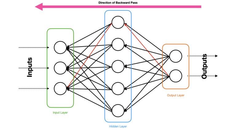
Figure 4: Propagation of information through a Neural Network during a Backward Pass. The loss \ell is computed at the output layer, and its effects are passed backwards through the network towards the input layer. One possible path, from output to input, is indicated in red.
The choice of \ell will be influenced by the type of problem we’re trying to solve. For classification problems, cross-entropy is a natural choice. For regression, the mean squared error (MSE) is often used. Since I will be building a regressor, and to simplify the calculations, I will choose a loss proportional to the MSE:
\ell = \frac{1}{2}\sum_k(y_k^{pred} – y_k^{true})^2 \propto \text{MSE} (5)
where k increments over each sample in our batch of training data.
As for the choice of f, I will pick the sigmoid activation function for the hidden layer:
f(z) = y = \frac{1}{1 + e^{-z}} (6)
The derivative of (6) is given by:
\frac{df}{dz}=y(1-y) (7)
A linear activation function will be used for the output layer:
f(z) = y = z (8)
where the derivative is given by:
\frac{df}{dz}=1 (9)
With all this decided, let’s now work through the backward pass for the example in Figure 4. Note that N is the number of samples in the training data:
- Output Layer (i=2):
- Compute the derivative of our loss function \frac{\partial\ell}{\partial \vec{y}^{pred}} = \frac{\partial\ell}{\partial \vec{y}^2} = \sum_k(\vec{y}_k^{pred} – \vec{y}_k^{true}) = \sum_k(\vec{y}_k^2 – \vec{y}_k^{true})
- Calculate \frac{\partial\ell}{\partial \vec{z}^2} = (\frac{\partial\ell}{\partial \vec{y}^2}) (\frac{df}{d\vec{z}^2}) = \frac{\partial\ell}{\partial \vec{y}^2}\odot\vec{1}. Note \odot denotes element-wise multiplication, and \vec{1} is a vector of 1’s
- Determine the derivative of the loss with respect to the weights in the output layer: \frac{\partial\ell}{\partial \bold{w}^2} = (\frac{\partial\ell}{\partial\vec{z}^2})( \frac{\partial\vec{z}^2}{\partial\bold{w}^2}) = (\frac{\partial\ell}{\partial \vec{y}^2}) (\vec{y}^1)^T. The superscript T denotes the transpose
- Determine the derivative of the loss with respect to the biases in the output layer: \frac{\partial\ell}{\partial\vec{b}^2} = \sum^N \frac{\partial\ell}{\partial\vec{z}^2}
- Hidden Layer (i=1):
- Work out the derivative of the loss with respect to the activation in this layer: \frac{\partial\ell}{\partial\vec{y}^1} = (\frac{\partial\ell}{\partial\vec{z}^2})(\frac{\partial\vec{z}^2}{\partial\vec{y}^1}) = \lbrack\bold{w}^2\rbrack^T(\frac{\partial\ell}{\partial \vec{y}^2})
- Determine \frac{\partial\ell}{\partial\vec{z}^1} = (\frac{\partial\ell}{\partial\vec{y}^1})(\frac{df}{d\vec{z}^1}), where \frac{df}{d\vec{z}^1} is described by equation (7)
- Calculate the derivative of the loss with respect to the weights in this layer: \frac{\partial\ell}{\partial\bold{w}^1} = (\frac{\partial\ell}{\partial\vec{z}^1})(\frac{\partial\vec{z}^1}{\partial\bold{w}^1}) = \frac{\partial\ell}{\partial\vec{z}^1}\vec{x}^T
- Determine the derivative of the loss with respect to the biases in the output layer: \frac{\partial\ell}{\partial\vec{b}^1} = \sum^N \frac{\partial\ell}{\partial\vec{z}^1}
- Weights Update: we can now update \bold{w}^1, \vec{b}^1, \bold{w}^2, and \vec{b}^2 by making use of the computed derivates. The mean of each derivative will be calculated over the N samples in the training data. A scalar learning rate \alpha will be used to control the size of the steps we take in weight space:
- \bold{w}^1 := \bold{w}^1 – \alpha \frac{1}{N} \frac{\partial\ell}{\partial\bold{w}^1}
- \vec{b}^1 := \vec{b}^1 – \alpha \frac{1}{N} \frac{\partial\ell}{\partial\vec{b}^1}
- \bold{w}^2 := \bold{w}^2 – \alpha \frac{1}{N} \frac{\partial\ell}{\partial\bold{w}^2}
- \vec{b}^2 := \vec{b}^2 – \alpha \frac{1}{N} \frac{\partial\ell}{\partial\vec{b}^2}
How Neural Networks Learn: Step-by-Step
We have now outlined all the terminology, and technical details, to understand the complete supervised learning procedure for Neural Networks. Let’s put everything together and outline the training algorithm point-by-point:
- \text{for e} = 1..epochs:
- \text{for b} = 1..batchs:
- Do a Forward Pass
- Do a Backward Pass
- Update the model weights
For each iteration in this algorithm, the networks weights will be adjusted to minimise the chosen loss function \ell. This is achieved by making use of a variant of gradient descent, which is increments along \ell in weight space to reach a minimum.
Note that our specific choice of optimisation algorithm will affect this procedure. For example, Batch Gradient Descent groups all the training data together, and as such the second loop over each batch is unnecessary. With Stochastic Gradient Descent, the same loop can be replaced by iterating over each sample in the training data.
The magnitude of the weight updates is controlled by the learning rate \alpha, which we introduced earlier. Early stopping is also possible, by defining a tolerance \tau below which the weight updates are not longer considered significant.
Final Remarks
In this post we have covered:
- The general approach to training supervised Neural Networks
- Illustrated the difference between Batch, Stochastic, and Mini-Batch Gradient Descent, and it’s impact on our learning procedure
- Worked through an example of the Forward Pass and Backward Pass, for a simple Neural Network architecture
I hope you enjoyed this article, and gained some value from it. If you have any questions or suggestions, please feel free to add a comment below. Your input is greatly appreciated.
Related Posts
Hi I'm Michael Attard, a Data Scientist with a background in Astrophysics. I enjoy helping others on their journey to learn more about machine learning, and how it can be applied in industry.