What is Stochastic Gradient Descent? 3 Pros and Cons

Gradient descent is a popular optimisation technique, and forms the basis of many learning algorithms. Perhaps most notably, Gradient Descent is used when training many types of neural networks. There are a few variants of this technique, but one of the most applicable when training on large datasets is Stochastic Gradient Descent. In this post, we’ll introduce this algorithm, and then go over 3 key advantages and disadvantages of this method. Finally, we’ll use 2 illustrative examples in Python to explore some of the aforementioned characteristics of Stochastic Gradient Descent. Anyone interested in using this approach, to train their model, should be aware of these points.

Table of Contents

What is Stochastic Gradient Descent? 3 Pros and Cons – image by Abi Plata

What is Stochastic Gradient Descent?

Generally speaking, gradient descent is an optimisation algorithm that attempts to find the best set of model parameters $\vec{w}$ (otherwise termed ‘weights‘) for a given problem. This is done by first selecting a loss function $\ell$ , by which the effectiveness of the model can be measured. As we improve the values of the weights, the model will perform better on the problem at hand. In other words, as $\vec{w}$ is optimised, $\ell$ will decrease. Therefore, we wish to find the set of model parameters that yields the minimum value of $\ell$ .

Some key points to make note of:

The approach we will take is iterative in nature, meaning we will repeat the stages of our algorithm a number of times as we ‘step’ towards our goal. This will not be an analytical solution.
We need to define a loss function $\ell$ for our problem, that is also a differentiable function of the model parameters $\vec{w}$ . If our problem, or choice of model, does not facilitate this, we cannot use gradient descent.

To move towards the minimum value of $\ell$ , we will compute the derivative with respect to the model parameters, $\partial\ell / \partial w$ . Since the derivative points towards the maximum value of $\ell$ in weight space, we will take a step in the opposite direction. The update rule is therefore defined by:

$\vec{w’} = \vec{w} – \alpha\frac{\partial \ell}{\partial w}$ (1)

where $\vec{w’}$ is the updated set of model parameters after a single step in our algorithm. The learning rate $\alpha$ is a hyperparameter, and controls how large the steps will be. Typical values for $\alpha$ range from 0.1 to 0.001.

We will repeat the update defined in (1) a number of times, until either the magnitude of the update falls below a tolerance threshold $\tau$ , or the maximum number repetitions has been made. At each step, we move towards the loss minimum in weight space. Figure 1 illustrates this scenario:

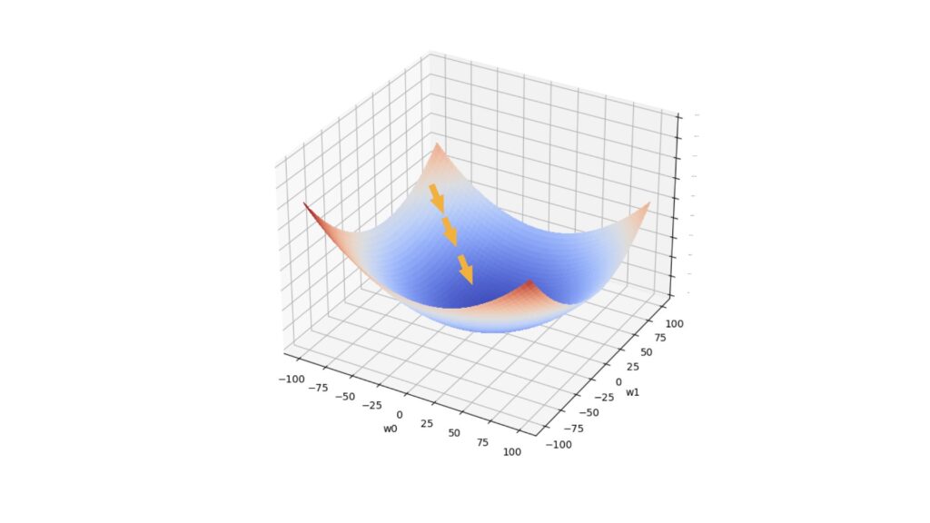
Figure 1: One possible path taken during the gradient descent algorithm. The horizontal axes represent 2 model parameters, whereas the vertical axis represents the loss value. The arrows indicate the movement taken during gradient descent, from a location of high loss to one with low loss.

With Stochastic Gradient Descent, we select a single random training sample to compute the model parameter updates, at each iteration. This algorithm consists of the following:

Choose values for the learning rate $\alpha$ , tolerance threshold $\tau$ , and number of epochs. The latter defines the maximum number of passes through the training data we will take in our procedure.
Initialise the values of the model parameters $\vec{w}$ .
for i = 1…\text{number of epochs}:
- randomly shuffle the training data
- for j = 1…\text{number of training samples}:
  - compute the derivative $\partial\ell / \partial w$ for training sample $j$ .
  - update the model parameters according to equation (1).
  - check if the magnitude of our update, $\alpha\frac{\partial \ell}{\partial w}$ , falls below $\tau$ . If so, exit the loop.

3 Pros of Stochastic Gradient Descent

There are a number of advantages to choosing Stochastic Gradient Descent, over other optimisation methods. Let’s outline 3 of the most important here.

I) Faster Convergence - Suitable for Larger Datasets

Since only a single training sample is used when computing the update $\alpha\frac{\partial \ell}{\partial w}$ , this technique can cycle through iterations while using minimal computational resources. This means we can take steps towards a minimum in weight space much faster, as compared to Batch Gradient Descent. Because of this property, Stochastic Gradient Descent is also an ideal choice for optimisation over a large dataset (where it is unpractical to load all the data into memory at runtime).

II) Able to Escape Local Minima

The aim of any gradient descent scheme is to find the global minimum in a defined space. However, problems can arise if local minima are present also (see Figure 3). In this scenario, we can get stuck in local minima, instead of correctly identifying the global minimum. Since Stochastic Gradient Descent is “stochastic“, there is a higher likelihood of escaping local minima (that aren’t too deep or broad) when compared with other methods. This feature will also be strongly dependant on the chosen learning rate $\alpha$ .

III) No Additional Hyperparameters

The number of hyperparameters is kept at a minimum, with no difference between this method and the simplest form of gradient descent. This facilitates ease-of-use for anyone wanting to make use of this algorithm.

3 Cons of Stochastic Gradient Descent

There are also some downsides to using Stochastic Gradient Descent in a given machine learning project. Let’s outline 3 of the most relevant.

I) Less Accurate Convergence

Since this approach is stochastic by nature, the path taken in weight space will be noisy. Depending on the size of the learning rate $\alpha$ , the algorithm can “bounce” around the minimum without zeroing-in on it.

II) More Complex Implementation

When compared with Batch Gradient Descent, this approach is more complex to implement since we must:

shuffle the training data for each epoch
loop through each training sample

The second point also implies we cannot vectorise our implementation. Solutions with higher complexity tend to increase the chances of making mistakes in the code. The fact that we cannot vectorise our solution means Stochastic Gradient Descent can be slower, compared to other variants of gradient descent, for smaller datasets.

III) Non-Deterministic

As already mentioned, this algorithm is stochastic in nature. Therefore, the output from any given optimisation run will have a random element to it. This randomness needs to be addressed when assessing the performance of any implementation of Stochastic Gradient Descent. This also implies that any learning algorithm trained in this way cannot be exactly duplicated.

Python Examples

I would now like to make some of the concepts discussed more tangible. Let’s work through an implementation of Stochastic Gradient Descent in Python, and test it with two different functions on a simple toy dataset. As a model to train, we will be making use of a simple linear regression.

MSE Loss Function

The mean squared error (MSE) is a common loss function used in regression problems. This is due to its simplicity, as well as to the fact that it is differentiable. Mathematically this is given by:

$\ell = \frac{1}{2N}\sum^N_i (y_{i,pred}-y_{i,true})^2$ (2)

where $y_{i,true}$ are the true target values, and $y_{i,pred}$ are the model predictions. For our purposes here, the latter quantity is given by: $y_{i,pred} = w_0 + w_1x_i$ , where $w_0$ is the bias, $x_i$ is a single predictor feature, and $w_1$ is the corresponding weight for this feature. Note that $\ell$ is a convex function of the model parameters. Figure 2 visualises this function below.

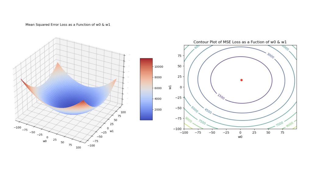
Figure 2: Surface plot (left) and contour plot (right) of the MSE loss. These plots were generated using a simple linear regression to produce predictions, and each plot was made as a function of the model parameters $\vec{w} = [w_0, w_1]$ . The red dot in the contour plot indicates the location of the global minimum.

Trigonometric Function

Let’s also define a more complicated function, that will produce a surface with many local minima and maxima. This function is defined by:

$\ell = \frac{1}{2N}\sum^N_i \theta_i^2sin\left(\frac{\pi \theta_i}{50}\right)$ (3)

where $\theta_i = (y_{i,pred}-y_{i,true})$ , and all the other parameters are the same as was defined for the MSE loss. Note that in this case, $\ell$ is non-convex. Figure 3 illustrates this function below:

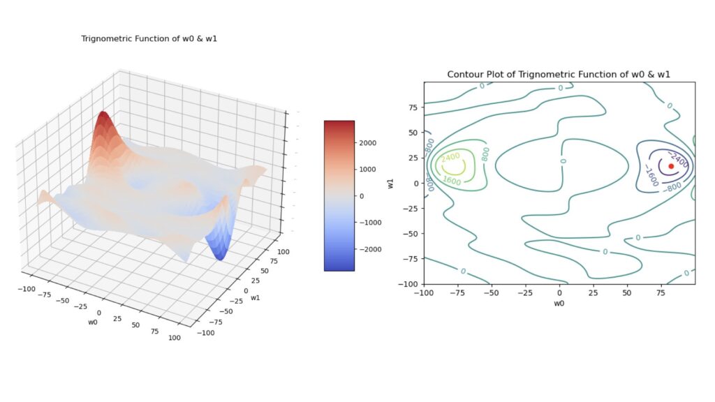
Figure 3: Surface plot (left) and contour plot (right) of the trigonometric function defined in (3). These plots were generated using a simple linear regression to produce predictions, and each plot was made as a function of the model parameters $\vec{w} = [w_0, w_1]$ . The red dot in the contour plot indicates the location of the global minimum.

Note that (3) is not a loss function used in machine learning, as the minimum of $\ell$ does not coincide with our desired state (i.e. $y_{i,pred}=y_{i,true}$ ). We will make use of it here simply because it provides a highly complex surface, with local maxima and minima, in weight space.

Implement Stochastic Gradient Descent

We can now put together a single Python function that will encompass the Stochastic Gradient Descent algorithm. This code will make use of the numpy package.

# imports
import numpy as np
import matplotlib.pyplot as plt
from matplotlib import cm
from matplotlib.ticker import LinearLocator
from typing import Callable, Tuple, Union
from sklearn.datasets import make_regression
from sklearn.metrics import mean_squared_error, mean_absolute_error

def stochastic_gradient_descent(X: np.array, 
                                y: np.array, 
                                model: Callable, 
                                Dloss: Callable, 
                                lr: float=0.1, 
                                epochs: int=500,
                                tol: float=1e-4,
                                verbose: bool=False) -> Tuple[np.array, list]:
    """
    Function to compute stochastic gradient descent for the provided training data using the input model & loss
    
    Inputs:
        Inputs:
        X       -> predictor values
        y       -> true target values
        model   -> function to compute model predictions
        Dloss   -> function to compute the derivate of the loss function in weight space
        lr      -> learning rate
        epochs  -> number of epochs to train
        tol     -> tolerance for early stopping
        verbose -> boolean to determine if extra information is printed out
        
    Output
        tuple containing a numpy array with the obtimised weights & list of the traversed path in weight space
    """
    # initialise weights 
    w_max  = 100.0
    w      = w_max*(np.random.rand(X.shape[1],1) - 0.5)
    w_path = []
    
    # cycle through epochs and update weights using batch gradient descent
    for _ in range(epochs):
        # shuffle data
        idx = np.random.permutation(X.shape[0])
        X   = X[idx,:]
        y   = y[idx].reshape(-1,1)
        # cycle through each sample in the training data
        for i in range(X.shape[0]):
            # store current weight values
            w_path.append(w.tolist())
            # make predictions
            yp = model(X[i,:],w)
            # compute the weights update & check tolerance
            dw = lr*Dloss(X[i,:],y[i],yp)
            w -= dw
            w = np.where(w > 100, 100, w)
            w = np.where(w < -100, -100, w)
            if np.linalg.norm(dw) < tol:
                break
            
    if verbose:
        yp = model(X,w)
        print(f"Error metrics: MSE = {mean_squared_error(y,yp):.2f}, MAE = {mean_absolute_error(y,yp):.2f}")
        print(f"Final weights: {float(w[0]):.2f}, {float(w[1]):.2f}")
    
    return (w, w_path)

The training data is composed of an array of predictor features X, and associated true target values y.
The input argument model is a function used to compute predictions at each iteration of the algorithm.
Dloss is another function, that computes the derivative of the (loss) function we are using.
The learning rate lr was termed $\alpha$ in (1). This controls the magnitude of the update step at each iteration.
The epochs argument defines the maximum number of times we pass through the entire set of training data. This is also the same as the number of iterations in our algorithm.
The tolerance tol, referred to as $\tau$ above, sets a lower bound for the size of our updates. The algorithm stops early if the magnitude of the update falls below this value.
The boolean argument verbose controls if performance metrics, and the final weights, are printed out once the algorithm finishes.

Let’s now write the remaining functions we’ll need for our tests. This will include a function for generating predictions from a linear regression model, as well as calculating the derivatives of (2) and (3):

def model(X: np.array, w: np.array) -> np.array:
    """
    Function to compute a linear model
    
    Inputs:
        X -> predictor values
        w -> weights
        
    Output:
        numpy array of predicted target values
    """
    return np.matmul(X,w)
    
def mse_gradient(X: np.array, y: np.array, yp: np.array) -> np.array:
    """
    Function to compute the derivative of the mse loss
    
    Inputs:
        X  -> predictor values
        y  -> true target values
        yp -> predicted target values
        
    Output
        numpy array containing the mse gradient
    """
    return (X*(yp-y)).reshape(-1,1)
    
def trig_gradient(X: np.array, y: np.array, yp: np.array) -> np.array:
    """
    Function to compute the derivative of the trignometric function
    
    Inputs:
        X  -> predictor values
        y  -> true target values
        yp -> predicted target values
        
    Output
        numpy array containing the trignometric gradient
    """
    theta = yp - y
    return ((theta*X)*(2*np.sin(np.pi*theta/50)+(np.pi*theta/50)*np.cos(np.pi*theta/50))).reshape(-1,1)

Create a Toy Dataset

I will make use of the make_regression function, from scikit-learn, to produce some data:

# make a simple regression dataset
X, y, coef = make_regression(n_samples=1000, n_features=1, noise=5, bias=2, coef=True, random_state=42)

Let’s visualise the data we’ve just created:

# plot the generated data
plt.scatter(X,y)
plt.xlabel('X')
plt.ylabel('y')
plt.title('Generated Dataset')
plt.show()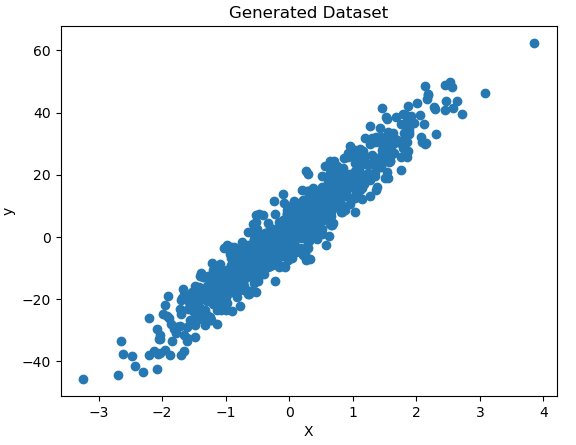

Figure 4: Generated toy dataset

Before testing our implementation on these data, let’s first add a column of 1’s to X to account for the bias parameter $w_0$ . Afterwards, we can also make note of the true value of $w_1$ :

# add bias term
b = np.ones((X.shape[0],1))
X = np.concatenate((b,X),axis=1)

# reshape true labels
y = y.reshape(-1,1)

# what is the model parameter?
coef

array(16.74825823)

Note that the true value of $w_0$ was set to 2.0 when we made the call to make_regression (see the bias input argument).

Stochastic Gradient Descent with MSE Loss

We can now test out our implementation using the MSE loss function, with 100 epochs and verbose set to True. All other parameters are set to their default values:

w, w_path = stochastic_gradient_descent(X, y, model, mse_gradient, epochs=100, verbose=True)

Error metrics: MSE = 24.53, MAE = 3.95
Final weights: 2.06, 16.86

The final weight values look quite good! Indeed they are very close to the true values of (2.0, 16.75).

I ran this code 3 separate times, to record the paths traversed by our implementation. Let’s take a look at how those trials turned out:

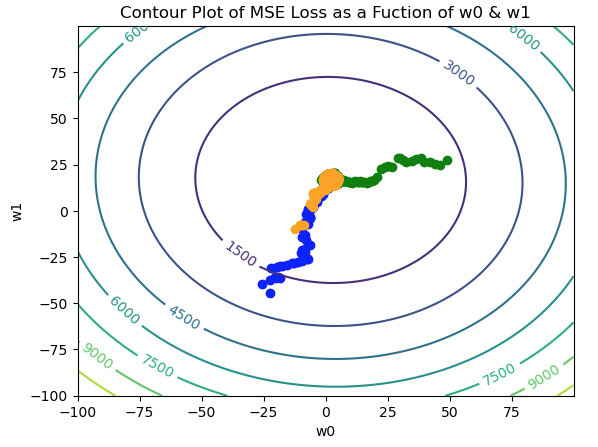
Figure 5: Contour plot for the MSE loss function, with 3 separate paths traversed in weight space. The paths are indicated in blue, green, and orange, and all converge to the global minimum near the center of the figure.

It is apparent in Figure 5 that each trial converges to the same point, regardless of the initial ( $w_0,w_1$ ) position. Note the paths traversed are quite noisy, as we would expect from a stochastic process.

Stochastic Gradient Descent with Trigonometric Function

Let’s now test out our implementation using the trigonometric function, described in equation (3). Here I’ll set the learning rate $\alpha$ to 0.01, and request 1000 epochs:

w, w_path = stochastic_gradient_descent(X, y, model, trig_gradient, lr=0.01, epochs=1000, verbose=True)

Error metrics: MSE = 1357.27, MAE = 36.48
Final weights: -34.49, 18.02

We can see the resulting weights deviate significantly compared to the true values. Unsurprisingly, the quality of the final generated predictions, reflected through the reported error metrics, is not as good as when we used the MSE loss.

Like before, I ran this experiment 3 times and recorded the paths traversed in weight space. Let’s look at these results:

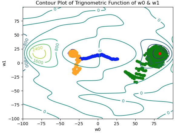
Figure 6: Contour plot for the trigonometric function described in (3), with 3 separate paths traversed in weight space. The paths are indicated in blue, green, and orange. Note the lack of convergence; there is no unique point on which all the paths converge. The true global minimum is indicated in red.

We can see the 3 paths indicated by the blue, orange, and green trails. With this function, finding the global minimum proves to be difficult, and the position settled upon by the algorithm is strongly dependent on the initial starting position. Two out of three paths (blue & orange) navigate towards a broad local minima in weight space. The green path manages to find the global minima after oscillating over the surrounding area.

Final Remarks

In this post we have covered:

What is the Stochastic Gradient Descent algorithm, and what it is used for.
3 Pros and Cons for using this variant of gradient descent.
How to implement Stochastic Gradient Descent in Python from scratch.
Explored how well does Stochastic Gradient Descent do when applied to convex and non-convex functions.

I hope you enjoyed this article, and gained some value from it. If you would like to take a closer look at the code presented here, please take a look at my GitHub. If you have any questions or suggestions, please feel free to add a comment below. Your input is greatly appreciated.

About Author

Hi I'm Michael Attard, a Data Scientist with a background in Astrophysics. I enjoy helping others on their journey to learn more about machine learning, and how it can be applied in industry.

Cookie	Duration	Description
cookielawinfo-checkbox-analytics	11 months	This cookie is set by GDPR Cookie Consent plugin. The cookie is used to store the user consent for the cookies in the category "Analytics".
cookielawinfo-checkbox-functional	11 months	The cookie is set by GDPR cookie consent to record the user consent for the cookies in the category "Functional".
cookielawinfo-checkbox-necessary	11 months	This cookie is set by GDPR Cookie Consent plugin. The cookies is used to store the user consent for the cookies in the category "Necessary".
cookielawinfo-checkbox-others	11 months	This cookie is set by GDPR Cookie Consent plugin. The cookie is used to store the user consent for the cookies in the category "Other.
cookielawinfo-checkbox-performance	11 months	This cookie is set by GDPR Cookie Consent plugin. The cookie is used to store the user consent for the cookies in the category "Performance".
viewed_cookie_policy	11 months	The cookie is set by the GDPR Cookie Consent plugin and is used to store whether or not user has consented to the use of cookies. It does not store any personal data.