As Decision Trees are supervised learning models, they cannot be directly applied to solve a clustering problem. However, they can be used after the application of a clustering algorithm, where the assigned clusters are treated as labels. The trained tree can then be easily visualised, to reveal the logic for how data are assigned to clusters. In this way, the trained Decision Tree can offer much more model transparency and interpretability to the clustering task.
Table of Contents
Why Should we use Decision Trees for Clustering Tasks?
Clustering falls under the domain of unsupervised machine learning: meaning that no labels or targets are known for the data. Instead, the task here is to try to identify unknown structure in the data. Clustering algorithms attempt to group different data points together, based on a measure of commonality. My previous article on the K-Means algorithm outlined one particular approach to the clustering problem.
One disadvantage for clustering algorithms, like K-Means, is that the results can be hard to explain or interpret. It can be difficult to comprehend why certain data points are assigned to a given cluster, versus any other. For the special case where our data contain only 2 features, the distributions in the data can be plotted, along with the cluster centroids found by the clustering algorithm.
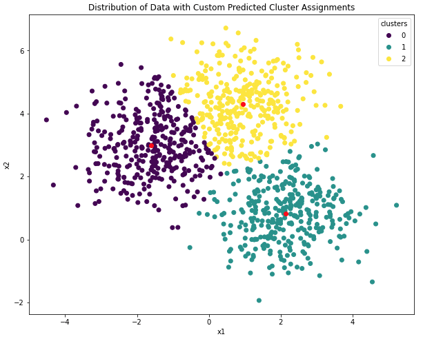
Figure 1: Illustration of clustering results for a dataset with only 2 features, x_1 and x_2. The data are grouped into 3 clusters. Cluster assignments are indicated by color, and cluster centroids are shown in red.
Figure 1 illustrates this case. Here, we can easily see that the proximity of the centroids to the data govern the cluster assignments. This type of scatter plot can be very helpful to explain the results to project stakeholders. The problem with this approach is that real-world datasets typically do not involve just 2 features; in reality hundreds if not thousands of features could be involved for a typical project. Under these circumstances, making scatter plots is simply not a practical solution to aid in explaining the results. In addition, although the scatter plot can show how the data are distributed, it still can be difficult to infer a clear reason as to why the clusters are located where they are.
Decision Trees are supervised machine learning algorithms that are fairly easy to visualise and interpret. Their interpretability is not affected by the dimensionality of the data either. As such, we can make use of a Decision Tree classifier to assist in explaining the clustering results.
Therefore, the overall procedure we will carry out is:
- Use a clustering algorithm (e.g. K-Means) to provide labels for an un-labelled dataset
- Train a Decision Tree on the data, using the original data as the predictor features and the clustering labels as our target
- Produce a flow chart of the trained Decision Tree, outlining how decisions are made and in what sequence, to yield predictions
Using a Decision Tree Classifier for Clustering in Python
Let’s now work through an actual example in Python. We will generate an unlabelled toy dataset, use K-Means to assign labels, and then apply a Decision Tree classifier to help us understand the results. To start let’s import all the packages necessary, and then generate the data by making use of make_blobs:
# imports
import numpy as np
from sklearn.tree import DecisionTreeClassifier, plot_tree
from sklearn.cluster import KMeans
from sklearn.datasets import make_blobs
from sklearn.metrics import accuracy_score, precision_score, recall_score, f1_score, mean_absolute_error
from sklearn.model_selection import train_test_split
import matplotlib.pyplot as plt

# make gaussian blobs
X, y, centers = make_blobs(n_samples=5000, centers=4, n_features=10, return_centers=True, random_state=42)
The data generated consist of 5000 samples with 10 features, that are grouped into 4 clusters. These are all contained in the output array X. The output y and centers are the true cluster assignments and centroid positions, respectively. Note there is no straight-forward way to visualise the clusters we have just generated, since they exist in 10-dimensional feature space.
I will refer to the 4 clusters as ‘cluster 0‘, ‘cluster 1‘, ‘cluster 2‘, and ‘cluster 3‘.
K-Means Clustering to Assign Labels
Let’s attempt to model the clusters generated, using K-Means from scikit-learn. I will take it for granted that we correctly know the number of clusters K to pick. I will specify that the training procedure should be done 20 times, to ensure we end up with a globally optimal solution:
# declare a k-means instance and train it on the data
kmeans = KMeans(n_clusters=4, random_state=42, n_init=20).fit(X)
# obtain cluster labelling on our data
y_kmeans = kmeans.predict(X)
I will try to figure out how well our clustering results are. First let’s see how well we found the centroids, and next we can check out our labelling:
# obtain the predicted centroids
centers_pred = kmeans.cluster_centers_
centers_pred
array([[-2.55860744, 8.96655941, 4.65750123, 1.95336489, -6.88301872,
-6.88442723, -8.84586538, 7.36514842, 2.03695905, 4.17960405],
[ 2.17173691, -6.58995626, -8.70377367, 8.99336112, 9.36044334,
6.14518609, -3.87511894, -8.0458794 , 3.71533124, -1.24329055],
[ 2.21862818, -7.21099843, -4.1732664 , -2.71633517, -0.86336467,
5.70631645, -6.00645567, 0.26412761, 1.80780239, -9.05101077],
[-9.5983904 , 9.39121113, 6.64885415, -5.72908004, -6.31014484,
-6.33581342, -3.91706392, 0.46949094, -1.34325217, -4.16683535]]) # what do the true centroids look like?
centersarray([[-2.50919762, 9.01428613, 4.63987884, 1.97316968, -6.87962719,
-6.88010959, -8.83832776, 7.32352292, 2.02230023, 4.16145156],
[-9.58831011, 9.39819704, 6.64885282, -5.75321779, -6.36350066,
-6.3319098 , -3.91515514, 0.49512863, -1.36109963, -4.1754172 ],
[ 2.23705789, -7.21012279, -4.15710703, -2.67276313, -0.87860032,
5.70351923, -6.00652436, 0.28468877, 1.84829138, -9.07099175],
[ 2.15089704, -6.58951753, -8.69896814, 8.97771075, 9.31264066,
6.16794696, -3.90772462, -8.04655772, 3.68466053, -1.19695013]]) K-Means focuses on finding clusters in the data, but will not necessarily reproduce the exact same labeling order. Let’s manually find the correct mapping, so we can compare the modelling results with the true values:
# mapping index
idx_pred_to_true = [0,3,2,1]
centers_pred[idx_pred_to_true,:]
array([[-2.55860744, 8.96655941, 4.65750123, 1.95336489, -6.88301872,
-6.88442723, -8.84586538, 7.36514842, 2.03695905, 4.17960405],
[-9.5983904 , 9.39121113, 6.64885415, -5.72908004, -6.31014484,
-6.33581342, -3.91706392, 0.46949094, -1.34325217, -4.16683535],
[ 2.21862818, -7.21099843, -4.1732664 , -2.71633517, -0.86336467,
5.70631645, -6.00645567, 0.26412761, 1.80780239, -9.05101077],
[ 2.17173691, -6.58995626, -8.70377367, 8.99336112, 9.36044334,
6.14518609, -3.87511894, -8.0458794 , 3.71533124, -1.24329055]]) # how accurate are our estimated centroids?
print(f'The mean absolute error between the predicted and true centroids is: \
{mean_absolute_error(centers,centers_pred[idx_pred_to_true,:]):.4f}')The mean absolute error between the predicted and true centroids is: 0.0194
The mean absolute error between the predicted and true centroid values is quite small! This indicates that K-Means has identified the correct locations for the cluster centres. Now let’s see how well the predicted cluster assignments match up with the true values, using standard classification error metrics:
# calibrate labelling
idx_0 = y_kmeans == 0
idx_1 = y_kmeans == 1
idx_2 = y_kmeans == 2
idx_3 = y_kmeans == 3
y_kmeans[idx_0] = 0
y_kmeans[idx_1] = 3
y_kmeans[idx_2] = 2
y_kmeans[idx_3] = 1

# how accurate are our cluster assignments?
acc = accuracy_score(y,y_kmeans)
pre = precision_score(y,y_kmeans,average='weighted')
rec = recall_score(y,y_kmeans,average='weighted')
f1  = f1_score(y,y_kmeans,average='weighted')
print(f'Accuracy score: {acc:.4f}')
print(f'Precision score: {pre:.4f}')
print(f'Recall score: {rec:.4f}')
print(f'F1 score: {f1:.4f}')
Accuracy score: 1.0000 Precision score: 1.0000 Recall score: 1.0000 F1 score: 1.0000
Okay, so it’s clear that K-Means has been able to reproduce the true clusters in the data! However, it isn’t clear how we can explain why a particular sample has been allocated to one cluster or another. Scatter plots, showing the data distribution and centroid locations, are not effective due to the high-dimensionality of the data. And even if we could produce these scatter plots, it still doesn’t answer the question of ‘why’ in a clear way.
Imagine a scenario where we take our trained K-Means model, and then try to generate predictions for some new data we have available. How can we explain the predicted cluster assignments for these data to stakeholders?
Decision Tree Classifier to Add Explainability
Here we will make use of the scikit-learn Decision Tree classifier to provide more explainability and transparancy to our analysis. We will treat the K-Means cluster assignments as our labels to be able to train the model. As this is a supervised learning problem, I will do a train-test split first so that our model evaluation can be done on a held-out test set. Twenty percent of the data will be reserved for testing.
# train-test split
X_train, X_test, y_train, y_test = train_test_split(X, y_kmeans, test_size=0.2, random_state=42, stratify=y_kmeans)

# declare a decision tree classifier instance and train it on the available data
clt = DecisionTreeClassifier(max_depth=5, random_state=42).fit(X_train, y_train)

# evaluate how well our classifier performs
y_pred = clt.predict(X_test)
acc    = accuracy_score(y_test,y_pred)
pre    = precision_score(y_test,y_pred,average='weighted')
rec    = recall_score(y_test,y_pred,average='weighted')
f1     = f1_score(y_test,y_pred,average='weighted')
print(f'Accuracy score: {acc:.4f}')
print(f'Precision score: {pre:.4f}')
print(f'Recall score: {rec:.4f}')
print(f'F1 score: {f1:.4f}')
Accuracy score: 1.0000 Precision score: 1.0000 Recall score: 1.0000 F1 score: 1.0000
Evidently the Decision Tree has managed to learn the labelling produced by K-Means. This now offers us a means to explain why samples are assigned to a given cluster and not others. Let’s plot the learned Decision Tree:
# plot tree
fig = plt.figure(figsize=(16,8))
_ = plot_tree(clt,
              filled=True,
              fontsize=10)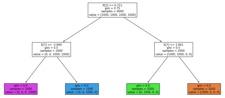
Figure 2: Structure of the trained Decision Tree for clustering. The coloured leaf nodes, from left to right, are for samples in cluster 3, cluster 2, cluster 1, and cluster 0.
Figure 2 offers a simple explanation as to why samples are labelled as they are. We can start at the root node, and then traverse the tree to see the decision rules that result in the cluster assignments. As an example, samples where feature x_2 is less than or equal to 0.311, and feature x_7 is greater than -3.849, are grouped together into cluster 2. It is interesting to note that although our data consist of 10 features, only 2 (x_2 & x_7) are used by the Decision Tree.
Final Remarks
This article outlined how to implement Decision Trees for clustering problems. My intention here was to provide a simple example outlining the use case for this approach. I hope that you enjoyed this content, and gained some value from it. If you have any questions or comments, please leave them below!
Related Posts
Hi I'm Michael Attard, a Data Scientist with a background in Astrophysics. I enjoy helping others on their journey to learn more about machine learning, and how it can be applied in industry.