In this post, we will cover the Gradient Boosting Regressor algorithm: the motivation, foundational assumptions, and derivation of this modelling approach. Gradient boosters are powerful supervised algorithms, and popularly used for predictive tasks.
Table of Contents
Motivation: Why Gradient Boosting Regressors?
The Gradient Boosting Regressor is another variant of the boosting ensemble technique that was introduced in a previous article. Development of gradient boosting followed that of Adaboost. In an effort to explain how Adaboost works, it was noted that the boosting procedure can be thought of as an optimisation over a loss function (see Breiman 1997). The original intent behind the development of gradient boosting was to take advantage of this realisation. The result was the creation of a general boosting algorithm that could handle a variety of loss functions, and constituent model types (i.e. “Weak Learners“). In practice, the constituent model type is normally a Decision Tree.
Following their initial development in the late 1990’s, gradient boosters have become the go-to algorithm of choice for online competitions and business machine learning applications. This is due to their versatility and superior predictive performance. For example, the Extreme Gradient Boosting package is a popular choice in industry, and a top performer in Kaggle competitions. More recent packages, such as LightGBM, are also gaining in popularity for a wide variety of practical problems.
In this article, I will specifically discuss the Gradient Boosting Regressor with Decision Trees, as outlined in Algorithm 3 of Friedman 2001.
Assumptions and Considerations
The following are a few key points to keep in mind when developing a Gradient Boosting Regressor algorithm:
- We want to build a model that addresses regression problems (continuous variables)
- The selected loss function must be differentiable
- Assumptions of the weak learner models, used to build the ensemble, need to be considered. For our purposes here, this means we need to consider the assumptions behind Decision Tree Regressors
- A feasible solution to our choice of fitting procedure, and weak learner model, must exist (see Algorithm 1, Step 4, in the following section)
General Gradient Boosting Regressor Algorithm
The general gradient boost algorithm described in Algorithm 1 of Friedman 2001 is outlined below. It is designed to handle any loss function \ell and weak learner f, so long as they adhere to the assumptions mentioned previously.
Let’s start with a few basic definitions. Our data will consist of predictors \bold{X} and targets \bold{y}. We will index through each unique sample in the data with n = 1..N. Likewise, we will index through each weak learner model, in our ensemble, with m = 1..M.
\bold{X} = \begin{bmatrix} \bold{x}_1 \\ \bold{x}_2 \\ . \\ . \\ \bold{x}_n \\ . \\ \bold{x}_N \end{bmatrix}, \bold{y} = \begin{bmatrix} y_1 \\ y_2 \\ . \\ . \\ y_n \\ . \\ y_N \end{bmatrix}, where \bold{x}_n \in R^{d}, y_n \in R (1)
f_m(\bold{x}_n) \in R (2)
\ell(y_n,f_m(\bold{x}_n)) \in R (3)
Here equations (1), (2), and (3) describe the data, weak learner model, and loss function, respectively. Note \bold{x}_n are the rows of matrix \bold{X}, and contain d features. Similarly, y_n are the scalar values of the column vector \bold{y}.
Like the other boosting algorithms discussed in previous articles, Gradient Boosting operates in a sequential, or stage-wise, manner. Each successive weak learner focuses on correcting the mistakes of the previous models. The mechanism used here to achieve this is steepest-decent. More specifically, the gradients of the loss function are computed and used as labels for f_m. The output from f_m is then set to be proportional to each “step” in the boosting procedure. Each iteration then approaches a minimum in the loss function space. The basic idea of this procedure is illustrated below:
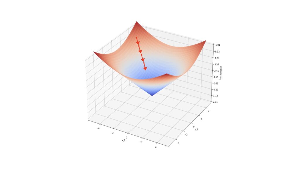
Depicted above is an example loss function \ell over a data space defined by (x_1,x_2). The red arrows indicate the gradients at specific locations on the surface defined by \ell. Each step in steepest-descent moves our loss value closer to the local minimum for this function.
With these ideas in place, let’s now outline the general gradient boosting regressor algorithm:
Algorithm 1: Gradient_Boost
- E_0(\bold{x}) = arg \: min_{y_{pred}}\sum_{n=1}^N\ell(y_n,y_{pred}) = E_0
- For m = 1 to M:
- Compute g_n = -\left[ \frac{\partial \ell (y_n,E(\bold{x}_n)) }{\partial E(\bold{x}_n) } \right] , where E(\bold{x}) = E_{m-1}(\bold{x}), for all n = 1..N
- \theta_m = arg \: min_{\theta,\beta}\sum_{n=1}^N \left[ g_n – \beta f(\bold{x}_n;\theta) \right]^2
- \rho_m = arg \: min_{\rho} \sum_{n=1}^N \ell(y_n,E_{m-1}(\bold{x}_n) +\rho f(\bold{x}_n;\theta_m) )
- E_m(\bold{x}) = E_{m-1}(\bold{x}) + \rho_m f(\bold{x};\theta_m)
We can go through each step in this algorithm and explain it in detail:
- Step 1. Initialise the ensemble to E_0
- Step 3. Compute the negative gradients of the loss function \ell with respect to the ensemble output at each data point \bold{x_n}. These point towards the local minimum in the space defined by \ell
- Step 4. Identify the weak learner f that most closely correlates with the gradients g_n, computed previously. Since the gradients are only defined on the points \bold{x}_n, this step is carried out in order to generalise the procedure to points \bold{x} that are not included in the training data. Although any fitting procedure could be used here, in Friedman 2001 least squares was chosen due to its computational properties
- Step 5. Determine the multiplier \rho_m for steepest-descent, making use of the weak learner f(\bold{x};\theta_m) found in the previous step
- Step 6. Increment the ensemble E_m using steepest-descent
Derivation of the Gradient Boosting Tree Regression Algorithm
We can now make Algorithm 1 more tangible by specifying the desired type of weak leaner f and loss function \ell. Let’s set these to be:
f(\bold{x};\theta) = \sum_{j=1}^Jb_jI(\bold{x} \in R_j) (4)
\ell(\bold{y},\bold{y}_{pred}) = |\bold{y} – \bold{y}_{pred}| (5)
Equation (4) is a decision tree with j = 1..J terminal regions defined by R_j, and b_j terminal values. Note that I is the identity matrix, and \theta = \{b_j,R_j\}_1^J. Equation (5) represents the absolute difference loss function.
Let’s first introduce equation (4) into Algorithm 1. Step 4 becomes fitting the decision tree on the negative gradients \bold{g} of the loss function, using least squares. Step 5 can now be updated as follows:
\rho_m = arg \: min_{\rho}\sum_{n=1}^N\ell(y_n,E_{m-1}(\bold{x}_n) + \rho\sum_{j=1}^Jb_jI(\bold{x}_n \in R_{jm}))
\{\gamma_{jm}\}_1^J = arg \: min_{\{\gamma_j\}_1^J}\sum_{n=1}^N\ell(y_n,E_{m-1}(\bold{x}_n)+\sum_{j=1}^J\gamma_jI(\bold{x}_n \in R_{jm}))
where \gamma_{jm} is a new optimum scaling factor over the possible \gamma_{j}=\rho b_j values for region j, at the m boosting step. Since the terminal regions produced by decision trees are disjoint, we can simplify this expression for a single value of j:
\gamma_{jm} = arg \: min_{\gamma}\sum_{\bold{x}_n \in R_{jm}}\ell(y_n,E_{m-1}(\bold{x}_n)+\gamma) (6)
Let’s proceed to update Step 6 from Algorithm 1:
E_m(\bold{x}) = E_{m-1}(\bold{x}) + \rho_m\sum_{j=1}^J b_{jm}I(\bold{x} \in R_{jm})
E_m(\bold{x}) = E_{m-1}(\bold{x}) + \sum_{j=1}^J \gamma_{jm}I(\bold{x} \in R_{jm}) (7)
Now that we have accounted for our choice of weak learner, it is time to address the loss function. We can now introduce equation (5) into Algorithm 1, starting with Step 1. To compute the argument minimum of \rho, we can take the derivative and set it to zero:
\frac{\partial E_0(\bold{x})}{\partial y_{pred}} = \sum_{n=1}^N sign(y_n – y_{pred}) = 0 \implies E_0(\bold{x}) = median(\bold{y}) (8)
So it is apparent that our choice of loss function leads us to initialise the ensemble with the median of the training labels. Moving on to Step 3, we can write:
g_n = -\left[ \frac{\partial \ell(y_n,E(\bold{x}_n))}{\partial E(\bold{x}_n)} \right] = +sign(y_n-E(\bold{x}_n)) (9)
Finally, we can insert (5) into (6), to complete our update of Step 5 of Algorithm 1:
\gamma_{jm} = arg \: min_{\gamma} \sum_{\bold{x}_n \in R_{jm}}(|y_n – E_{m-1}(\bold{x}_n) – \gamma|)
To find the argument minimum, let’s compute the dervative over the sum, and set it to zero:
\frac{\partial}{\partial \gamma} \sum_{\bold{x}_n \in R_{jm}}|y_n – E_{m-1}(\bold{x}_n) – \gamma| = \sum_{\bold{x}_n \in R_{jm}} sign(y_n – E_{m-1}(\bold{x}_n) – \gamma_{jm}) = 0
\implies \gamma_{jm} = median_{\bold{x}_n \in R_{jm}}(y_n – E_{m-1}(\bold{x}_n)) (10)
Our updates are complete. What we have now is the third algorithm from Friedman 2001.
Algorithm 3: LAD_TreeBoost
The training procedure is as follows:
- E_0(\bold{x}) = median(\bold{y}) = E_0
- For m=1 to M:
- g_n = sign(y_n – E_{m-1}(\bold{x}_n)), for all n=1..N
- Fit a J terminal node decision tree to \{ g_n,\bold{x}_n \}_1^N, and obtain the set of terminal regions \{ R_{jm} \}_1^J
- \gamma_{jm} = median_{\bold{x}_n \in R_{jm}}(y_n – E_{m-1}(\bold{x}_n)), for all j = 1..J
- E_m(\bold{x}) = E_{m-1}(\bold{x}) + \sum_{j=1}^J \gamma_{jm}I(\bold{x} \in R_{jm})
This procedure will yield E_0, the sets of parameters \{ R_{jm} \} and \{ \gamma_{jm} \}, and the set of M trained decision trees. The general flow through the algorithm can be visualised as below:
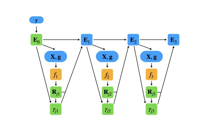
This example consists of a gradient boosting regressor of 3 elements. Here green elements are the learned model parameters from training, and orange represent the weak learners of the ensemble. Data, gradients, and ensemble states at each iteration, are indicated in blue. The data are used to calculate the gradients \bold{g} and produce trained decision trees f_m. These are then used, along with the value for E_{m-1}, to compute the weights \gamma_{jm}. Finally, the ensemble is updated to E_m, and the next iteration begins.
Predictions from this ensemble, on a set of input data \bold{x}', can then be obtained by:
- Initialise the ensemble to E_0
- For m=1 to M:
- E_m(\bold{x}') = E_{m-1}(\bold{x}') + \sum_{j=1}^J \gamma_{jm}I(\bold{x}' \in R_{jm})
- Return E_M(\bold{x}')
Final Remarks
In this article you have learned:
- The motivation behind the Gradient Boosting Regressor algorithm, and when it was developed
- The general Gradient Boosting Regressor algorithm, for abstract loss functions and weak learners
- How to derive the LAD_TreeBoost algorithm, which is an implementable form of Gradient Boosting
I hope you enjoyed this article, and gained value from it. In the next article, I will implement the LAD_TreeBoost algorithm in Python from scratch.
If you have any questions or suggestions, please feel free to add a comment below. Your input is greatly appreciated.
Related Posts
Hi I'm Michael Attard, a Data Scientist with a background in Astrophysics. I enjoy helping others on their journey to learn more about machine learning, and how it can be applied in industry.
Great article!!
Glad you enjoyed it!
[…] See my articles on Bagging, Random Forest, Adaboost Classification, Adaboost Regression, and Gradient Boost for examples of […]
[…] of the specific problem. However a rough rule of thumb is that if a top-performing algorithm (e.g. Gradient Boost) does not show improved performance for increasing training set size, it may be a good idea to try […]
[…] can also look at my blog articles, where is describe the mathematical details of the Gradient Boosting Algorithm, as well as how this algorithm can be implemented in Python from […]
[…] can also look at my blog articles, where is describe the mathematical details of the Gradient Boosting Algorithm, as well as how this algorithm can be implemented in Python from […]