Understanding the Adaboost Regression Algorithm

In this post, we will describe the Adaboost regression algorithm. We will start with the basic assumptions and mathematical foundations of this algorithm, and work straight through to an implementation in Python from scratch.

Table of Contents

Motivation: What is a Adaboost Regressor?

In this post, we will describe the Adaboost regression algorithm. We will start with the basic assumptions and mathematical foundations of this algorithm, and work straight through to an implementation in Python from scratch. Adaboost stands for “Adaptive Boosting”, and this was the first boosting technique to gain wide popularity. The algorithm was originally developed by Freund and Schapire 1997.

In a previous post, I introduced the concept of boosting regression and built a simple boosting regressor in Python. I also compared its performance to a single Decision Stump and Random Forest. That model made use of a fixed learning rate during training. The learning rate was used to update the sample weights during each training iteration.

Here we will dispense with the learning rate parameter entirely. Instead, the sample weights will be set dynamically at each training step. This is the reason why the algorithm is termed “adaptive”. In this way, we can build a boosting regressor with consistently better performance. Like all other ensemble techniques, Adaboost combines multiple simple learning models (i.e. “Weak Learners”) into a single powerful regressor. Note that the specific implementation covered in this article follows the Adaboost.R2 algorithm, described in Drucker 1997.

Assumptions and Considerations

Some key points to keep in mind when using a Adaboost.R2 regressor:

It is important to make the ensemble of sufficient size to obtain good results
Assumptions of the weak learner, used to build the ensemble, should be considered. In general, the weak learner should be a very “simple” model
Outliers can cause problems if present in the data. Boosting regressors can place too much weight on these samples, which will affect performance
Since boosting is a sequential algorithm, it can be slow to train. A long training period can affect the scalability of the model

Derivation of a Adaboost Regression Algorithm

Let’s begin to develop the Adaboost.R2 algorithm. We can start by defining the weak learner, loss function, and available data. We will assume there are a total of $N$ samples available in the data, and our ensemble consists of $M$ weak learners. We will index through each unique sample in the data with $n = 1..N$ . Likewise, we will index through each weak learner model, in our ensemble, with $m = 1..M$ .

$\bold{X} = \begin{bmatrix} \bold{x}_1 \\ \bold{x}_2 \\ . \\ . \\ \bold{x}_n \\ . \\ \bold{x}_N \end{bmatrix}$ , $\bold{y} = \begin{bmatrix} y_1 \\ y_2 \\ . \\ . \\ y_n \\ . \\ y_N \end{bmatrix}$ , where $\bold{x}_n \in R^{d}$ , $y_n \in R$ (1)

$f_m(\bold{x}_n) \in R$ (2)

$\ell(f_m(\bold{x}_n),y_n) \in [0,1]$ (3)

Here equations (1), (2), and (3) describe the data, weak learner model, and loss function, respectively. Note $\bold{x}_n$ are the rows of matrix $\bold{X}$ , and contain $d$ features. Similarly, $y_n$ are the scalar values of the column vector $\bold{y}$ .

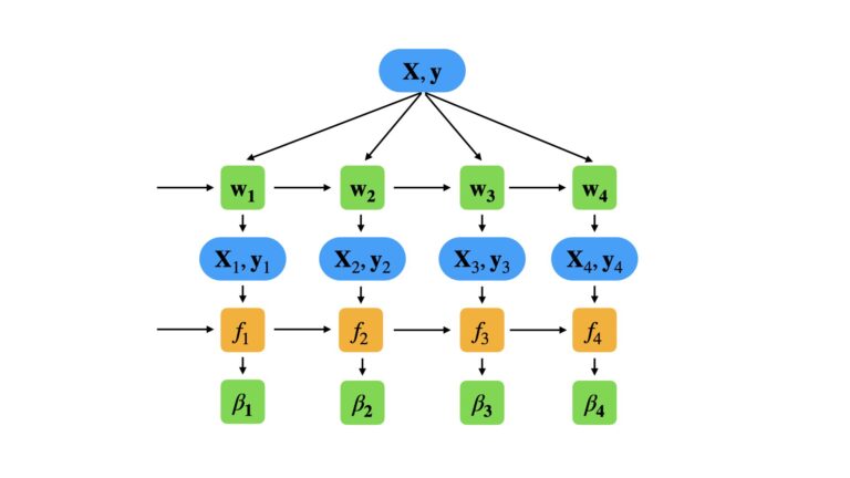
With these definitions in place, we can now specify our training procedure. Like all other boosting methods, Adaboost.R2 is a sequential algorithm. The weak learners $f_m$ are trained one after the other on data ( $\bold{X}_m,\bold{y}_m$ ), which are sampled from ( $\bold{X},\bold{y}$ ) with replacement. The sample weights $\bold{w}$ are updated at each step in the sequence, in order to place more focus on mistakes made during the previous step. A model confidence measure $\beta_m$ also needs to be assigned to the $m$ ^th weak learner, in order to properly combine it with the rest of the ensemble. We can illustrate this procedure below, for a small ensemble consisting of $M = 4$ weak learners:

The specific steps in our training procedure are as follows:

for $n = 1..N$ , initialise sample weights as $w_n^1 = 1$
for m = 1..M calculate:
1. calculate the sample probabilities $p_n = w_n^m/\sum_n{w_n^m}$ for all $n$ . Using $p_n$ , select $N$ samples from ( $\bold{X},\bold{y}$ ) with replacement. These data are termed ( $\bold{X}_m,\bold{y}_m$ )
2. fit $f_m$ to $(\bold{X}_m,\bold{y}_m)$
3. compute the loss $\ell_n$ for each sample. To do this, we will obtain predictions $\bold{y}’$ from $f_m$ on all the available predictors in the training data ( $\bold{X}$ ). Any function can be used for the loss, so long as it adheres to (3)
4. compute the average loss $\bar{\ell}=\sum_n\ell_np_n$ . If $\bar{\ell} \ge 0.5$ , terminate the training loop early
5. calculate the confidence measure $\beta_m = \frac{\bar{\ell}}{1-\bar{\ell}}$ . A low $\beta_m$ implies high confidence in the prediction
6. update the sample weights by $w_n^{m+1} = w_n^m\beta_m^{1-\ell_n}$

The update procedure outlined by step 6 places more weight on samples that have larger differences between observations and predictions. In this way, each subsequent weak learner focuses more on the mistakes made by the previous model in the ensemble.

We can elaborate further on the loss function $\ell_n$ mentioned in step 3. The original paper (Drucker 1997) defines three functional forms:

Linear: $\ell_n = \frac{|y’_n – y_n|}{D}$ (4)

Square: $\ell_n = \frac{|y’_n – y_n|^2}{D^2}$ (5)

Exponential: $\ell_n = 1 – exp\{\frac{-|y’_n – y_n|}{D}\}$ (6)

where $D$ is the supremum of $|y’_n - y_n|$ , for all $n = 1..N$ .

For a given input $\bold{x}^*$ , predictions can now be obtained with the following procedure:

generate predictions from each weak learner $y_m^* = f_m(\bold{x}^*)$
sort the predictions according to $y_1^* < y_2^* < \dots < y_M^*$ . Make note of the associated $\beta_m$ for each $y_m^*$ , and retain this association in the sorted order
consider an integer $K$ that is $K \le M$ . For $k = 1..K$ , begin summing $log(\frac{1}{\beta_k})$ until the following inequality is satisfied:

$\sum_k^{K : K \le M} log(\frac{1}{\beta_k}) \ge \frac{1}{2}\sum_m^Mlog(\frac{1}{\beta_m})$ (7)

The prediction generated from the smallest $K$ ^th machine, that satisfies (7), is the ensemble prediction. Note that this value, $y_K^*$ , is the weighted median of the predicted values $y_m^*$ .

Implementation of a Adaboost Regressor in Python

Now we will proceed to encapsulate the Adaboost Regression algorithm, described in the previous section, into a single Python class. Our implementation will depend on the numpy and typing packages, as well as the clone function from sklearn.base.

import numpy as np
from typing import Dict, Any, List, Tuple
from sklearn.base import clone

Let’s start with the class definition, initialiser, and destructor functions:

## adaboost regressor ##
class AdaBoostRegressor(object):
    #initialiser
    def __init__(self, 
                 weak_learner : Any, 
                 n_elements : int = 100, 
                 loss : str = 'linear') -> None:
        self.weak_learner    = weak_learner
        self.n_elements      = n_elements
        self.loss_type       = loss
        self.f               = []
        self.model_weights   = []
        self.mean_loss       = []
        
    #destructor
    def __del__(self) -> None:
        del self.weak_learner
        del self.n_elements
        del self.loss_type
        del self.f
        del self.model_weights
        del self.mean_loss

__init__(self, weak_learner, n_elements, loss) : This is the initialiser function that is called whenever a class instance is created. The argument weak_learner is a model object that will be used to build the ensemble, and is assumed to follow the structure of a standard scikit-learn model. n_elements is an integer value that defines how many weak learners will be used to build the ensemble. Finally, loss is a string argument that can take the following values: ‘linear‘, ‘square‘, and ‘exponential‘. This defines the loss function to use, according to equations (4), (5), and (6).
__del__(self) : Here we have the destructor function, which is called whenever a class instance is deleted. It cleans up resources allocated to the instance.

Let’s now define the private functions that implement the possible losses for this class:

    #private linear loss function
    def __linear_loss(self,y_pred : np.array, y_train : np.array) -> np.array:
        #compute the square loss function
        loss = np.abs(y_pred - y_train)
        loss /= np.max(loss)
        #return computed loss
        return(loss)
    
    #private square loss function
    def __square_loss(self,y_pred : np.array, y_train : np.array) -> np.array:
        #compute the square loss function
        loss = np.abs(y_pred - y_train)
        loss = np.power(loss/np.max(loss),2)
        #return computed loss
        return(loss)    
    
    #private exponential loss function
    def __exponential_loss(self,y_pred : np.array, y_train : np.array) -> np.array:
        #compute the square loss function
        loss = np.abs(y_pred - y_train)
        loss = 1 - np.exp(-loss/np.max(loss))
        #return computed loss
        return(loss)

__linear_loss(self, y_pred, y_train) : This function implements equation (4) for the training procedure.
__square_loss(self, y_pred, y_train) : This function implements equation (5) for the training procedure.
__exponentional_loss(self, y_pred, y_train) : This function implements equation (6) for the training procedure.

Note that for practical purposes, this supremum is treated as the maximum absolute difference between $y’_n$ and $y_n$ . We can proceed now to define the remaining private functions for this class:

    #private loss function
    def __compute_loss(self,y_pred : np.array, y_train : np.array) -> np.array:
        #select correct loss function
        if self.loss_type == 'linear':
            loss = self.__linear_loss(y_pred,y_train)
        elif self.loss_type == 'square':
            loss = self.__square_loss(y_pred,y_train)
        elif self.loss_type == 'exponential':
            loss = self.__exponential_loss(y_pred,y_train)
        else:
            raise ValueError('Incorrect loss type entered, must be linear, square, or exponential')
        #return computed loss
        return(loss)
    
    #private function to compute model weights
    def __compute_beta(self, p : np.array, loss : np.array) -> Tuple[float,float]:
        #compute the mean loss
        mean_loss = np.sum(np.multiply(loss,p))
        #calculate beta
        beta = mean_loss/(1-mean_loss)
        #store model weights & mean loss
        self.model_weights.append(np.log(1.0/beta))
        self.mean_loss.append(mean_loss)
        #return computed beta & mean loss
        return(beta,mean_loss)

    #private function to compute weighted median
    def __weighted_median(self, y_samp : np.array) -> np.array:
        #sort sample predictions column-wise
        samp_idx = np.argsort(y_samp,axis=0)
        sorted_y = y_samp[samp_idx.T]
        sorted_y = np.array([sorted_y[i,:,i] for i in range(sorted_y.shape[0])]).T
        #sort the model weights according to samp_idx
        sorted_mw = np.array(self.model_weights)[samp_idx]
        #do cumulative summation on columns
        cumsum_mw = np.cumsum(sorted_mw,axis=0)
        #solve inequality
        pred_idx = cumsum_mw >= 0.5*cumsum_mw[-1,:]
        pred_idx = pred_idx.argmax(axis=0)
        #return weighted medians
        return(sorted_y[pred_idx].diagonal())

__compute_loss(self, y_pred, y_train) : This function handles the call to the appropriate loss function, as requested by the user. If the request is not one of the currently supported loss functions, an error is raised.
__compute_beta(self, p, loss) : The calculation of $\bar{\ell}$ and $\beta_m$ , as defined in steps 4 and 5 of our training procedure, are done here. Both $\bar{\ell}$ and $log(\frac{1}{\beta_m})$ are stored internally.
__weighted_median(self, y_samp) : The final two steps of our prediction procedure are handled here. The output are the weighted medians of $y_m^*$ .

At this stage, we can implement our training function:

    #public function to train the ensemble
    def fit(self, X_train : np.array, y_train : np.array) -> None:
        #initialise sample weights, model weights, mean loss, & model array
        w                  = np.ones((y_train.shape[0]))
        self.f             = []
        self.model_weights = []
        self.mean_loss     = []
        #loop through the specified number of iterations in the ensemble
        for _ in range(self.n_elements):
            #make a copy of the weak learner
            model = clone(self.weak_learner)
            #calculate probabilities for each sample
            p = w/np.sum(w)
            #sample training set according to p
            idx = np.random.choice(y_train.shape[0],y_train.shape[0],replace=True,p=p)
            X = X_train[idx]
            y = y_train[idx]
            #fit the current weak learner on the boostrapped dataset
            model.fit(X,y)
            #obtain predictions from the current weak learner on the entire dataset
            y_pred = model.predict(X_train)
            #compute the loss
            loss = self.__compute_loss(y_pred,y_train)
            #compute the adaptive weight
            beta,mean_loss = self.__compute_beta(p,loss)
            #check our mean loss
            if mean_loss >= 0.5:
                break
            #update sample weights
            w *= np.power(beta,1-loss)
            #append resulting model
            self.f.append(model)

fit(self, X_train, y_train) : In this public function the entire training procedure, outlined in the previous section, is implemented. The trained weak learner models, $f_m$ , are stored internally.

Implementation of the remaining functions for this class are now described:

    #public function to return mean training loss
    def get_loss(self) -> List:
        return(self.mean_loss)
 
    #public function to return model parameters
    def get_params(self, deep : bool = False) -> Dict:
        return {'weak_learner':self.weak_learner,
                'n_elements':self.n_elements,
                'loss':self.loss_type}

    #public function to generate predictions
    def predict(self, X_test : np.array) -> np.array:
        #obtain sample predictions for each memeber of the ensemble
        y_samp = np.array([model.predict(X_test) for model in self.f])
        #do weighted median over the samples
        y_pred = self.__weighted_median(y_samp)
        #return predictions
        return(y_pred)

get_loss(self) : The mean loss, stored internally during training, is returned by this public function.
get_params(self, deep) : This is a public function to return the input arguments when an instance of this class is created. This function is required when using AdaBoostRegressor object instances in scikit-learn functions.
predict(self, X_test) : Here we have a public function used to generated predictions from the trained ensemble. The input X_test is a set of predictors upon which the model output will be based. The prediction procedure from the previous section is implemented here.

Measuring the Performance of our Adaboost Regressor

Now we’ll test out the performance of our custom-built adaboost regressor! Note that this boosting algorithm makes no explicit assumptions regarding the form of the weak learner described by equation (2). The only constraint placed on the weak learner is that its return values are limited to the real number line $R$ .

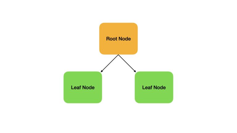
In practice, a Decision Stump is almost always used as the weak learner. This is a special type of Decision Tree with only one split:

We will begin our analysis by importing all the required packages for our work:

## imports ##
import numpy as np
import pandas as pd
import seaborn as sn 
from typing import Dict, Any, List, Tuple
from sklearn.base import clone
import matplotlib.pyplot as plt
from sklearn.datasets import load_diabetes
from sklearn.model_selection import cross_validate
from sklearn.tree import DecisionTreeRegressor
from sklearn.metrics import mean_squared_error,mean_absolute_error,make_scorer
from sklearn.ensemble import RandomForestRegressor

Data Import and Exploration

The data we will use here is the Diabetes Dataset available through scikit-learn. Let’s load these data into our work environment:

## load regression dataset ##
dfX,sy = load_diabetes(return_X_y=True,as_frame=True)

A full description of this dataset is available here. The features in the predictor dataframe dfX are as follows:

age age in years
sex
bmi body mass index
bp average blood pressure
s1 tc, total serum cholesterol
s2 ldl, low-density lipoproteins
s3 hdl, high-density lipoproteins
s4 tch, total cholesterol / HDL
s5 ltg, possibly log of serum triglycerides level
s6 glu, blood sugar level

The target series sy is a quantitative measure of disease progression one year after baseline.

As our next step, let’s make some plots to illustrate the distributions in the available data:

## histogram plot of predictors & targets ##
df = dfX.copy()
df['Target'] = sy
df.hist(bins=30,figsize=(15,10))
plt.show()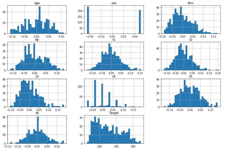

## boxplot of predictors ##
df.boxplot(column=dfX.columns.values.tolist(),figsize=(15,10))
plt.show()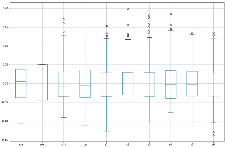

The features follow various different distributions, and many show the presence of outliers. Outliers are apparent for bmi, s1, s2, s3, s4, s5, and s6. Note that the predictors have already been mean centered and scaled by the standard deviation such that the sum of squares equals 1.

To what degree are these features correlated? Let’s take a look at a heat map of the Pearson correlation:

## plot the pearson correlation for our data ##
fig, ax = plt.subplots(figsize = (8, 8)) 
dfCorr  = df.corr() 
sn.heatmap(dfCorr) 
plt.show()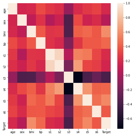

The heatmap indicates some interesting points:

s3 appears to be consistently anti-correlated with all other features + Target
s1 & s2 appear to be highly correlated
The Target does not appear to be strongly correlated/anti-correlated with any single feature over the others

Investigate Training Loss

I now want to look at how the training loss evolves as weak learners are added to the ensemble. The training loss has an odd shape, since we divide by the supremum. As we iterate through he ensemble, it is expected that the loss should start off near 0.0 and progress towards 0.5. At a loss of 0.5, the update rule for the sample weights no longer works ( $\beta_m = 1.0$ ), and as such training stops. The loss is expected to evolve this way since with each successive weak learner, the difference between the supremum and $abs(y^{pred}_i – y^{true}_i)$ , for all $i$ , should shrink.

Let’s start with initialising the weak learner, which will be a regression decision stump:

## initialize a weak learner ##
weak_m = DecisionTreeRegressor(max_depth=1)

We will train the model on the raw data features, since decision trees can typically handle data with little preprocessing:

## train the adaboost classifier ##
rgr = AdaBoostRegressor(weak_learner=weak_m, loss='linear')
rgr.fit(dfX.values,sy.values)

## get linear loss ##
linear_loss = rgr.get_loss()

## train the adaboost classifier ##
rgr = AdaBoostRegressor(weak_learner=weak_m, loss='square')
rgr.fit(dfX.values,sy.values)

## get square loss ##
square_loss = rgr.get_loss()

## train the adaboost classifier ##
rgr = AdaBoostRegressor(weak_learner=weak_m, loss='exponential')
rgr.fit(dfX.values,sy.values)

## get exponential loss ##
exp_loss = rgr.get_loss()

## plot the training loss ##
plt.plot(linear_loss,label='linear')
plt.plot(square_loss,label='square')
plt.plot(exp_loss,label='exponential')
plt.title('Training Loss by Boosting Iteration')
plt.xlabel('Number of Component Trees')
plt.ylabel('Loss')
plt.legend()
plt.show()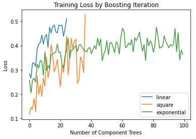

The linear and square loss functions terminate at around 20 and 40 weak learners, respectively. It is at this point where the loss reaches 0.5 from an initial low value. The exponential loss does not reach 0.5, for the default number of weak learners in our Adaboost implementation (100). As such, training does not terminate early when using this loss function.

Regardless of the choice of loss function, the implementation appears to be functioning as we would expect. The loss starts at a low value, and proceeds towards 0.5 as more weak learner models are added to the ensemble. Once the loss reaches 0.5, training is terminated.

Cross Validation Analysis

Note: rerunning these cells will show some fluctuation in the results

Here I will use 10-fold cross-validation to measure the performance of the Adaboost regressor. I will use the linear loss, and set the maximum number of elements to 20:

## define the scoring metrics ##
scoring_metrics = {'mse' : make_scorer(mean_squared_error), 
                   'mae': make_scorer(mean_absolute_error)}
                   
## perform cross-validation for linear loss & n_elements = 20 ##
#define the model
rgr = AdaBoostRegressor(weak_learner=weak_m, loss='linear', n_elements=20)
#cross validate
dcScores = cross_validate(rgr,dfX.values,sy.values,cv=10,scoring=scoring_metrics)
#report results
print('Mean MSE: %.2f' % np.mean(dcScores['test_mse']))
print('Mean MAE: %.2f' % np.mean(dcScores['test_mae']))

Mean MSE: 3782.54

Mean MAE: 52.02

We can compare these results with the Adaboost regressor available from scikit-learn:

## import adaboost regressor from scikit-learn ##
from sklearn.ensemble import AdaBoostRegressor

## perform cross-validation for linear loss & n_elements=20 ##
#define the model
rgr = AdaBoostRegressor(base_estimator=weak_m, loss='linear', n_estimators=20)
#cross validate
dcScores = cross_validate(rgr,dfX.values,sy.values,cv=10,scoring=scoring_metrics)
#report results
print('Mean MSE: %.2f' % np.mean(dcScores['test_mse']))
print('Mean MAE: %.2f' % np.mean(dcScores['test_mae']))

Mean MSE: 3827.65

Mean MAE: 52.40

We can see there is a small difference between the two Adaboost models. Note both Adaboost regressors are based on the same R2 algorithm.

Now let’s compare our results with a lone weak learner, and a Random Forest Regressor with 20 constituent weak learners:

#cross validate
dcScores = cross_validate(weak_m,dfX.values,sy.values,cv=10,scoring=scoring_metrics)
#report results
print('Mean MSE: %.2f' % np.mean(dcScores['test_mse']))
print('Mean MAE: %.2f' % np.mean(dcScores['test_mae']))

Mean MSE: 4751.55

Mean MAE: 56.68

## perform cross-validation for n_elements=20 & max_depth=1 ##
#define the model
rgr = RandomForestRegressor(n_estimators=20,max_depth=1)
#cross validate
dcScores = cross_validate(rgr,dfX.values,sy.values,cv=10,scoring=scoring_metrics)
#report results
print('Mean MSE: %.2f' % np.mean(dcScores['test_mse']))
print('Mean MAE: %.2f' % np.mean(dcScores['test_mae']))

Mean MSE: 3935.18

Mean MAE: 52.12

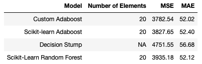
The Adaboost regressors produce the best overall results, with both our custom implementation, and the one available from scikit-learn, yielding similar numbers. The Random Forest of 20 Decision Stumps performs a bit worse with respect to Adaboost. The lone Decision Stump shows the worst overall performance.

Final Remarks

In this article you have learned:

The motivation behind the Adaboost regression algorithm, and when it was developed
A derivation of the Adaboost.R2 algorithm
How to implement the Adaboost regression algorithm in Python from scratch
How our implementation of Adaboost compares against open-source, scikit-learn regression models

I hope you enjoyed this article, and gained some value from it. If you would like to take a closer look at the code presented here, please take a look at my GitHub. If you have any questions or suggestions, please feel free to add a comment below. Your input is greatly appreciated.

5 2 votes

Article Rating

3 Comments

Oldest

Newest Most Voted

Inline Feedbacks

View all comments

indra

1 year ago

hi it is a veru helpful article, thanks alot

Author

insidelearningmachines

Reply to indra

Glad you enjoyed the article!

Build a Decision Tree in Python from Scratch - Inside Learning Machines

[…] through the use of ensembles. See my articles on Bagging, Random Forest, Adaboost Classification, Adaboost Regression, and Gradient Boost for examples of […]

Cookie	Duration	Description
cookielawinfo-checkbox-analytics	11 months	This cookie is set by GDPR Cookie Consent plugin. The cookie is used to store the user consent for the cookies in the category "Analytics".
cookielawinfo-checkbox-functional	11 months	The cookie is set by GDPR cookie consent to record the user consent for the cookies in the category "Functional".
cookielawinfo-checkbox-necessary	11 months	This cookie is set by GDPR Cookie Consent plugin. The cookies is used to store the user consent for the cookies in the category "Necessary".
cookielawinfo-checkbox-others	11 months	This cookie is set by GDPR Cookie Consent plugin. The cookie is used to store the user consent for the cookies in the category "Other.
cookielawinfo-checkbox-performance	11 months	This cookie is set by GDPR Cookie Consent plugin. The cookie is used to store the user consent for the cookies in the category "Performance".
viewed_cookie_policy	11 months	The cookie is set by the GDPR Cookie Consent plugin and is used to store whether or not user has consented to the use of cookies. It does not store any personal data.