What is Cross Validation?

A natural question to ask, when building any predictive model, is how good are the predictions? Having a clear, quantitative measure for the expected model performance, is a key element to any machine learning project.  

Cross validation is a family of techniques used to measure the effectiveness of predictions, generated from machine learning models. Broadly speaking, cross validation involves splitting the available data into train and test sets. The model is fitted on the training set, and then performance is measured over the test set. In this way, we estimate the effectiveness of our model on ‘unseen data’ (i.e. data not included when training the model). The approach to making these train/test splits is what defines one cross validation technique from the other.

In this post, we’ll cover the most common approaches to cross validation in machine learning. These can be divided into two categories: Exhaustive and Non-Exhaustive. Exhaustive techniques involve dividing the data into all possible train/test combinations for evaluation. This approach is more robust against bias, but is also more computationally expensive. Non-Exhaustive techniques do not include dividing the data into all possible train/test combinations. This approach is much faster to complete, but can be subject too much more bias.

Illustrative Examples

We will begin by covering Exhaustive cross validation techniques. Afterwards, Non-Exhaustive approaches will be discussed. 

To help with the following subsections on Exhaustive and Non-Exhaustive cross validation, a couple of simple, illustrative datasets will be used. These will be introduced at the beginning of each subsection. Although the examples used here will represent classification problems, most of the techniques described will work equally well in the case of regression (stratified methods are not applicable to regression problems).

Exhaustive Cross Validation in Machine Learning

Here we will make use of a series of animal images. Each image is labelled as to whether the particular animal is a mammal or not. Let’s take a look at these “data”:

cross validation

There are a series of four images, each of which is labelled with a check mark (mammal) or X (not a mammal). In this setup, the images can been seen as the predictor variables, while the check marks/X’s represent the labels.

Leave p Out Cross Validation

Leave p Out Cross Validation (LpOCV) involves using p samples as the test set, and the remainder n – p for training. Note that n is the total number of samples in the dataset. This is done over all possible ways to sample the p data points for testing. This requires running ’n choose p’ (nCp) tests. 

As an example of this approach, consider the case where p = 2 for our animal image dataset. In this case, 4C2 = 6 separate tests need to be run:

cross validation

It is apparent, from the figure above, that all possible pair combinations are represented in the test sets. The results from the individual tests can be combined, to yield a final performance measure. The combination will typically involve a mean or median calculation. For larger values of n and p, this technique can require a lot of tests!

Leave One Out Cross Validation

Leave One Out Cross Validation (LOOCV) is fundamentally the same as LpOCV, except that we set p = 1. This approach requires nC1 = n tests, which is computationally less intensive when compared to LpOCV.

Within the context of our animal image dataset, we get the following setup for LOOCV:

cross validation

Like the LpOCV case, the results from the individual tests can be combined, to yield a final performance measure.

Non-Exhaustive Cross Validation in Machine Learning

For this subsection, I will augment the animal image dataset, introduced earlier, to include a total of 10 images: 

cross validation

Like before, these “data” consist of a series of images that serve as the predictor variables. Each image has a label corresponding to whether the animal is a mammal or not. The labels are either a check mark (mammal) or X (non-mammal). There are a total of 5 mammal images, and 5 non-mammal images, included in these data. Therefore we are working with a balanced classification dataset.

Hold Out

This is by far the simplest approach to testing a machine learning model’s performance. Hold Out consists of sampling a certain percentage of the available data, say 10% to 30%, for testing. These sampled data are excluded while training the model. Using our animal image dataset, this looks like:

cross validation

The vertical line, between the rooster and monkey, indicates the separation between training and test sets. This simple division makes computation quick, however bias can be a major problem. Bias can be introduced in cases where the resulting train and test sets do not effectively represent the actual data-generating process being investigated. This is typically a problem where the available dataset is small. Large datasets, where the cropped test set is still sufficiently representative of the underlying data distribution, may fair well with this method.

An additional concern, specific to classification problems, is the question of selection bias. Depending on how the test set is selected, the resulting train and test sets may not have the same proportion of classes as the totality of all the available data. This is illustrated in the example above: overall there are the same number of mammals as non-mammals in our dataset. However, the train set only contains 2/6 mammals, while the test set has 3/4 mammals. As such, neither is effectively representative of our data as a whole.

Stratified Hold Out

Stratified Hold Out is a technique meant to address the problem of selection bias in Hold Out applied to classification problems. It is essentially the same as Hold Out, except that we ensure that the same proportion of classes is allocated to both the train and test sets. This can be illustrated as follows:

cross validation

Note that we still have a single train and test set, as with Hold Out. However, each now are balanced in terms of the class labels. Both the train and test sets have 50% mammal images, and 50% non-mammal images. It is important to highlight that with stratification, the proportion of class labels in the train and test sets is made to be the same as in the entire dataset.

K-Fold Cross Validation

As a further step against bias in our procedure, we can divide the available data into K non-overlapping partitions. This partitioning of the data is illustrated below for K = 5:

cross validation

We can then evaluate the model performance as follows:

for k = 1..K:

  • train the model on the data contained in all partitions p where p \ne k
  • test the trained model on the data contained in partition k
  • record the test results for the kth iteration

The K test results can then be combined, either through the mean or median calculation. 

This procedure is termed K-Fold Cross Validation. It is more robust against bias when compared to Hold Out, since we are effectively resampling the train and test sets K times. And although K-Fold Cross Validation is not as thorough as LpOCV, it is also not as computationally intensive. Typical values of K are 5 or 10.

Stratified K-Fold Cross Validation

Bias can be introduced in K-Fold Cross Validation, if the classes present in the K partitions are not in the same proportions as seen in the overall dataset. If you look at the visualisation used for K-Fold Cross Validation above, you will see that the classes do not occur in the 50%:50% proportions for all but the k=3 partition. This implies that selection bias will be introduced when modeling this dataset.

Stratified K-Fold Cross Validation is meant to treat for selection bias when analysing classification problems. This procedure is essentially the same as K-Fold Cross Validation, except that the classes are stratified in each of the K folds. This is visualised below:

cross validation

We can see now that each of the K folds contain the same percentage of mammal and non-mammal images, as in the complete dataset. As such, selection bias will not be a concern when testing over the k = 1..K folds.

Implementing Cross Validation in Python

Now we can work through the cross validation techniques discussed above, in Python. Let’s get started by importing a few packages: 

## imports ##
import time
import numpy as np
from sklearn.datasets import make_classification
from sklearn.metrics import accuracy_score, precision_score, recall_score, f1_score, make_scorer
import matplotlib.pyplot as plt
from sklearn.tree import DecisionTreeClassifier

We can now create a small toy classification dataset to work with, using scikit-learn’s make_classification function:

## create a classification dataset ##
X,y = make_classification(n_samples=100, 
                          n_features=10, 
                          n_informative=5, 
                          n_redundant=2, 
                          n_classes=2, 
                          weights=[0.4,0.6],
                          random_state=42)

These data consist of 100 samples, 2 class labels, and a total of 10 predictive features. I have specified that 5 of the 10 features are informative, and 2 are redundant. I have also set the class weights to be 0.4 and 0.6.

Let’s make a couple plots to better understand the data we have generated:

## plot the distribution of the predictor features ##
plt.boxplot(X)
plt.xlabel('features')
plt.ylabel('values')
plt.title('Distributions in Predictor Features')
plt.show()
cross validation
## plot the distribution of the labels ##
plt.bar(['0','1'],[y[y==0].shape[0], y[y==1].shape[0]])
plt.xlabel('classes')
plt.ylabel('frequency')
plt.title('Frequency of Label Classes')
plt.show()
cross validation

The box plot reveals all the predictor features are roughly centred close zero, and have approximately similar spreads. A few outliers are also present. The bar plot illustrates the imbalance in class frequencies, as was set  by the weights argument to make_classification.

Finally, let’s now initialise a classifier to fit to these data. I will use a Decision Tree in this case, with default input parameters:

## initialise classifier model ##
model = DecisionTreeClassifier()

I will quantify the results from each cross validation run using the accuracy, precision, recall, and F1 score metrics. 

Leave p Out Cross Validiation

We can import the module for Leave p Out Cross Validation from scikit-learn:

## import LpOCV functionality ##
from sklearn.model_selection import LeavePOut

Let’s now initialise an instance, where p = 4 samples will be held out for each test. We will then run through the LpOCV procedure:

## initialise cv instance ##
lpo = LeavePOut(4)
print("Number of splits: ",lpo.get_n_splits(X))
Number of splits:  3921225
## iterate through each split and evaluate ##
y_true = []
y_pred = []
start_time = time.time()
for train_idx, test_idx in lpo.split(X):
    #extract train & test sets
    X_train, X_test = X[train_idx], X[test_idx]
    y_train, y_test = y[train_idx], y[test_idx]
    #fit the model
    model.fit(X_train,y_train)
    #store results
    y_true.extend(list(y_test))
    y_pred.extend(list(model.predict(X_test)))
print('Time duration of LpOCV computation: ',time.time()-start_time)
Time duration of LpOCV computation:  3062.1051337718964

The LpOCV calculation will require ~3.9 million tests! Note that the computation time has been recorded. Total time duration to run LpOCV was approximately 3062 seconds, or ~51 minutes. Let’s now complete our evaluation to quantify the results:

print('accuracy score: %.2f' % accuracy_score(y_true,y_pred))
print('precision score: %.2f' % precision_score(y_true,y_pred))
print('recall score: %.2f' % recall_score(y_true,y_pred))
print('f1 score: %.2f' % f1_score(y_true,y_pred))
accuracy score: 0.79
precision score: 0.82
recall score: 0.83
f1 score: 0.83

I repeated this analysis 3 times, to check for consistency in the results. We can now take a look at the results:

cross validation

It is apparent that the results are completely consistent across the 3 separate runs. This consistency suggests that selection bias is not a concern in this case.

Leave One Out Cross Validation

Let’s import the module for Leave One Out Cross Validation from scikit-learn:

## import LOOCV functionality ##
from sklearn.model_selection import LeaveOneOut

Now we can initialise an instance, and run through the LOOCV procedure:

## initialise cv instance ##
loo = LeaveOneOut()
print("Number of splits: ",loo.get_n_splits(X))
Number of splits:  100
## iterate through each split and evaluate ##
y_true = []
y_pred = []
start_time = time.time()
for train_idx, test_idx in loo.split(X):
    #extract train & test sets
    X_train, X_test = X[train_idx], X[test_idx]
    y_train, y_test = y[train_idx], y[test_idx]
    #fit the model
    model.fit(X_train,y_train)
    #store results
    y_true.extend(list(y_test))
    y_pred.extend(list(model.predict(X_test)))
print('Time duration of LOOCV computation: ',time.time()-start_time)
Time duration of LOOCV computation:  0.08274579048156738

The total time duration to run LOOCV was only 0.08 seconds. In addition, the number of tests required was 100.  Both of these metrics are dramatically less than in the LpOCV case. Let’s now complete our evaluation:

print('accuracy score: %.2f' % accuracy_score(y_true,y_pred))
print('precision score: %.2f' % precision_score(y_true,y_pred))
print('recall score: %.2f' % recall_score(y_true,y_pred))
print('f1 score: %.2f' % f1_score(y_true,y_pred))
accuracy score: 0.77
precision score: 0.81
recall score: 0.80
f1 score: 0.81

Like in the LpOCV case, I repeated this analysis 3 times, to check for consistency in the results. The results from each of the runs is summarised below:

cross validation

These results are still quite consistent, however some fluctuations are apparent over the different runs. This variation is due to the fewer number of tests being conducted for each run. The LpOCV results show no variation since they are averaged over ~3.9 million tests, in contrast to LOOCV, where the same averaging is done over just 100 tests.

In general, all the metrics recorded are a bit lower than when using LpOCV, which yields the impression of slightly poorer model performance.

Hold Out

We can accomplish Hold Out by making use of the train_test_split function from scikit_learn. Let’s import this functionality, and do Hold Out with 20% of the data being reserved for testing:

## import hold out CV functionality ##
from sklearn.model_selection import train_test_split

## run hold out cross validation ##
start_time = time.time()
X_train, X_test, y_train, y_test = train_test_split(X, y, test_size=0.20)
model.fit(X_train,y_train)
y_pred = model.predict(X_test)
print('Time duration of Hold Out computation: ',time.time()-start_time)
Time duration of Hold Out computation:  0.0020160675048828125
print('accuracy score: %.2f' % accuracy_score(y_test,y_pred))
print('precision score: %.2f' % precision_score(y_test,y_pred))
print('recall score: %.2f' % recall_score(y_test,y_pred))
print('f1 score: %.2f' % f1_score(y_test,y_pred))
accuracy score: 0.70
precision score: 0.75
recall score: 0.75
f1 score: 0.75

Unsurprisingly, the computation time is very fast, just 0.002 seconds. Like before, I will repeat the analysis over the course of 3 separate runs:

cross validation

What stands out immediately is the fluctuations in our results. Clearly we don’t have consistent results using Hold Out on these data! This is an example of the effects of selection bias: depending on what samples are selected to be part of the test set, the results can vary considerably. It would be difficult to draw any conclusions, regarding model performance on these data, using this approach.

Stratified Hold Out

Let’s try to improve upon our Hold Out results, by attempting Stratified Hold Out. We can go ahead and implement that now, by feeding our labels to the stratify argument in train_test_split:

## run stratified hold out cross validation ##
start_time = time.time()
X_train, X_test, y_train, y_test = train_test_split(X, y, test_size=0.20, stratify=y)
model.fit(X_train,y_train)
y_pred = model.predict(X_test)
print('Time duration of Stratified Hold Out computation: ',time.time()-start_time)
Time duration of Stratified Hold Out computation:  0.0024750232696533203
print('accuracy score: %.2f' % accuracy_score(y_test,y_pred))
print('precision score: %.2f' % precision_score(y_test,y_pred))
print('recall score: %.2f' % recall_score(y_test,y_pred))
print('f1 score: %.2f' % f1_score(y_test,y_pred))
accuracy score: 0.75
precision score: 0.77
recall score: 0.83
f1 score: 0.80

The computation time is still 0.002 seconds, like with Hold Out. I will now repeat this analysis over the course of 3 separate runs:

cross validation

Large fluctuations in the result metrics are still apparent, like with Hold Out. Let’s check if K-Fold Cross Validation can yield more consistent results?

K-Fold Cross Validation

There is a scikit-learn function to implement K-Fold Cross Validation in Python. Let’s import that now:

## import k-fold CV functionality ##
from sklearn.model_selection import cross_validate

We can now setup our scoring metrics, run the cross validation procedure, and print the mean results over the K folds:

## define the scoring metrics ##
scoring_metrics = {'accuracy' : make_scorer(accuracy_score), 
                   'precision': make_scorer(precision_score),
                   'recall': make_scorer(recall_score),
                   'f1': make_scorer(f1_score)}
                   
## run k-fold cross validation ##
start_time = time.time()
dcScores = cross_validate(model,X,y,cv=10,scoring=scoring_metrics)
print('Time duration of K-fold CV computation: ',time.time()-start_time)
Time duration of K-fold CV computation:  0.03740215301513672
#report results
print('Mean accuracy: %.2f' % np.mean(dcScores['test_accuracy']))
print('Mean precision: %.2f' % np.mean(dcScores['test_precision']))
print('Mean recall: %.2f' % np.mean(dcScores['test_recall']))
print('Mean f1: %.2f' % np.mean(dcScores['test_f1']))
Mean accuracy: 0.76
Mean precision: 0.80
Mean recall: 0.82
Mean f1: 0.80

I have chosen K=10 in this particular case. The computation time is significantly larger than was the case with Hold Out, but is still only a fraction of a second. Like with the previous examples, I have recorded the results from 3 separate runs:

cross validation

It is clear that these results are far more consistent between runs, when compared to (Stratified) Hold Out. Nonetheless, variation is still seen between runs. We can try to improve these results with Stratified K-Fold Cross Validation.

Stratified K-Fold Cross Validation

We will need to import StratifiedKFold from scikit-learn, in addition to cross_validate:

## import stratification functionality ##
from sklearn.model_selection import StratifiedKFold

We will now run the cross validation procedure, and print the mean results over the K folds:

## run stratified k-fold cross validation ##
start_time = time.time()
dcScores = cross_validate(model,X,y,cv=StratifiedKFold(10),scoring=scoring_metrics)
print('Time duration of Stratified K-fold CV computation: ',time.time()-start_time)
Time duration of Stratified K-fold CV computation:  0.038410186767578125
#report results
print('Mean accuracy: %.2f' % np.mean(dcScores['test_accuracy']))
print('Mean precision: %.2f' % np.mean(dcScores['test_precision']))
print('Mean recall: %.2f' % np.mean(dcScores['test_recall']))
print('Mean f1: %.2f' % np.mean(dcScores['test_f1']))
Mean accuracy: 0.78
Mean precision: 0.82
Mean recall: 0.82
Mean f1: 0.81

Once again I have set K=10. The computation time is virtually unchanged from K-Fold Cross Valdiation. I will again illustrate the results from 3 separate runs:

cross validation

While there is still some variation between runs, it looks to be less than the case with K-Fold Cross Validation. 

Final Remarks

We have covered many of the most popular methods of cross validation in machine learning. Of the coding examples considered in this post, it appears that LpOCV, LOOCV, and Stratified K-Fold cross validation yield the most consistent results. This implies that these approaches are the most resilient against bias in our testing procedure.

It is important to note that neither LpOCV or LOOCV scale well with larger datasets. Even with our toy dataset of 100 samples, running LpOCV took over 50 minutes to complete just one run. And LOOCV runs as many tests as there are samples in the dataset. As such, when attempting cross validation for a machine learning project, (Stratified) K-Fold cross validation is probably a good option to start with. Ultimately, the choice of cross validation technique will depend upon the amount of data available, computational resources, time constraints, and desired minimal precision and accuracy of the test results.

Related Posts

5 1 vote
Article Rating
Subscribe
Notify of
guest

5 Comments
Oldest
Newest Most Voted
Inline Feedbacks
View all comments
Abigail Plata
Abigail Plata
1 year ago

Great article!! Keep them coming

trackback

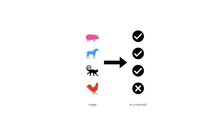
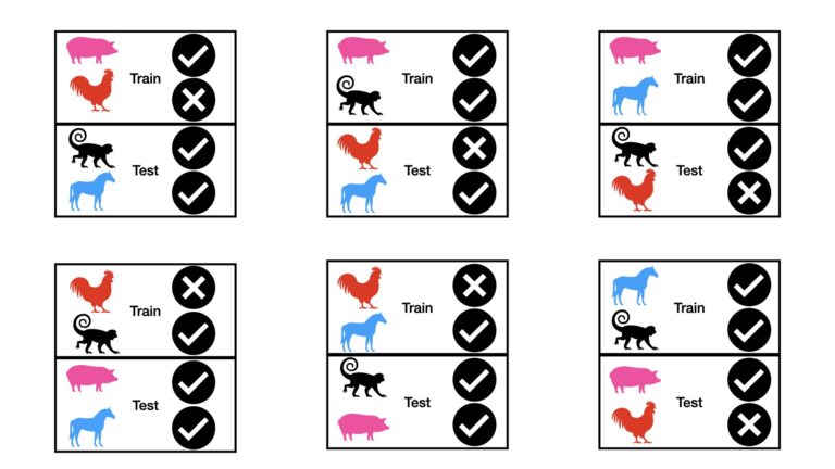
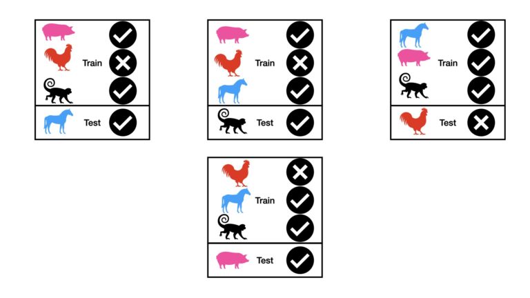
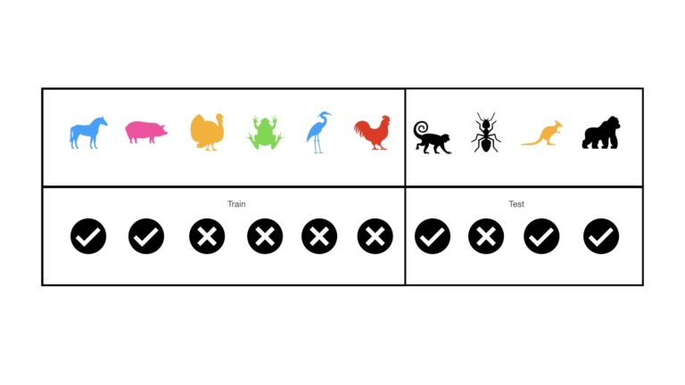
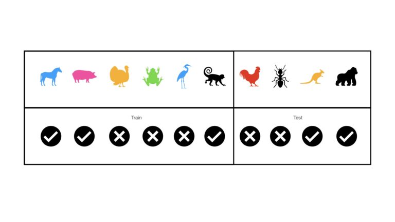
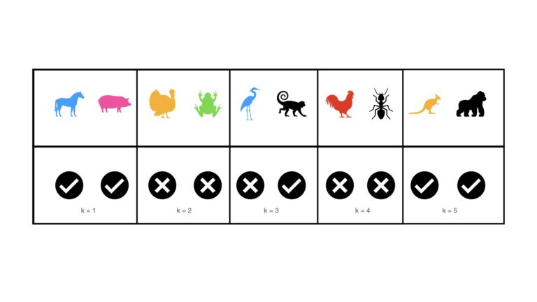
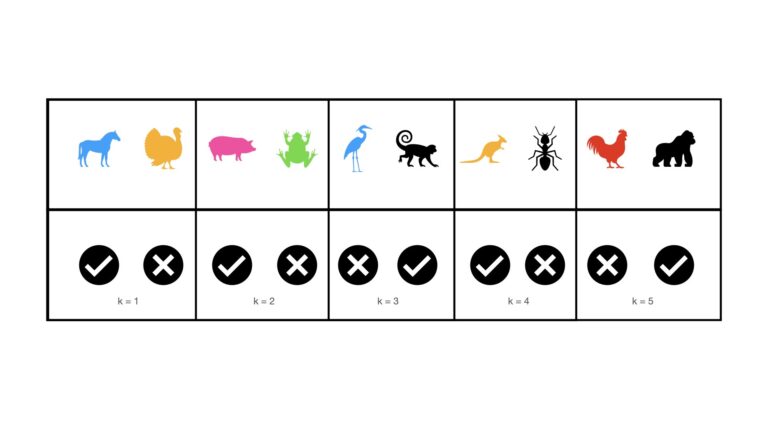
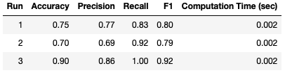
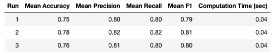
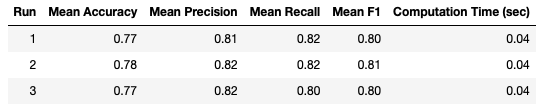
[…] as to which method we use, it is best practice to evaluate each hyperparameter configuration with Cross-Validation.  More specifically, it is typical to make use of K-Fold Cross-Validation to determine the […]

trackback

[…] via the ordering in the pipeline. In addition, pipelines facilitate a data scientist in performing cross-validation over an entire modelling project that is composed of various steps (pre-processing, modelling, […]

trackback

[…] entire Pyspark data processing sequences. In addition, pipelines enable data scientists to perform cross-validation over an entire modeling project that is composed of various steps (pre-processing, modeling, […]

5
0
Would love your thoughts, please comment.x
()
x