We can tune hyperparameters in Decision Trees by comparing models trained with different parameter configurations, on the same data. An optimal model can then be selected from the various different attempts, using any relevant metrics. There are several different techniques for accomplishing this task. Three of the most popular approaches for hyperparameter tuning include Grid Search, Randomised Search, and Bayesian Search.
Table of Contents
Why Tune Hyperparameters in Decision Trees?
Like most machine learning algorithms, Decision Trees include two distinct types of model parameters: learnable and non-learnable. Learnable parameters are calculated during training on a given dataset, for a model instance. The model is able to learn the optimal values for these parameters are on its own. In essence, it is this ability that puts the “learning” into machine learning.
By contrast, non-learnable parameters cannot be inferred from the training data. Instead they must be set outside of the training process. Often these parameters define a specific architecture for a given model (e.g. number of trees in a Random Forest).
Normally, the non-learnable parameters are referred to as the Hyperparameters of a model. The learnable parameters can simply be referred to as the parameters, or weights.
In Decision Trees, the parameters consist of the selected features f, and their associated split points s, that define how data propagate through the nodes in a tree. Some of the most common hyperparameters include:
- Choice of splitting loss function, used to determine (f,s) at a given node
- Maximum depth of the tree, which sets a hard limit on how much branching can occur
- Minimum number of samples for a split, which places a lower bound on how much data must enter a node for it not to be considered a leaf node during training
- Maximum number of leaf nodes, a value used to set an upper bound on the number of terminal points in the tree
Optimising the values of the hyperparameters, for a specific task, will often lead to superior model performance. Put simply, the Decision Tree will be able to make better predictions on unseen data. Many of these hyperparameters will perform a regularisation function during training, and thereby help to prevent overfitting.
What Methods are Used to Tune Hyperparameters?
In this post, we’ll use 3 of the most popular choices for hyperparameter tuning. These include:
- Grid Search: This involves an exhaustive search through a list of all possible hyperparameter values to try. Every possible combination is tried, and then the best performing model can be selected. While this option tends to perform well, it is computationally expensive
- Randomised Search: In this approach, a random set of samples are selected from the hyperparameter space. We can define the hyperparameter space with lists (like in Grid Search), or with statistical distributions. Randomised Search is much more computationally efficient, but can yield lower quality results if we are not careful with the parameter space definition
- Bayesian Search: Here we build a probabilistic model to identify the best set of hyperparameters. The hyperparameter space is defined by statistical distributions. We can further influence how the tuning performs through a careful selection of prior distributions. This method is also computationally efficient, but it is more complex to use or explain, when compared with Grid Search or Randomised Search
Regardless as to which method we use, it is best practice to evaluate each hyperparameter configuration with Cross-Validation. More specifically, it is typical to make use of K-Fold Cross-Validation to determine the performance of a model with a certain set of hyperparameter values. This reduces any possible bias introduced by the way we split our training and validation data sets.
Python Coding Examples
We can now work through some examples to tune hyperparameters in Decision Trees. I will attempt to tune classification and regression Decision Trees on a toy dataset. Each of the methods described in the previous section will be tried.
Note that we will be working with the scikit-learn Decision Tree implementations. The hyperparameters I will attempt to optimise include:
- criterion (this is the splitting loss function mentioned previously)
- max_depth
- min_samples_split
- max_leaf_nodes
Let’s start by importing all the necessary packages:
# imports
import time
import numpy as np
from sklearn.datasets import make_classification, make_regression
from sklearn.model_selection import train_test_split
from sklearn.tree import DecisionTreeClassifier, DecisionTreeRegressor
from sklearn.model_selection import GridSearchCV, RandomizedSearchCV
from sklearn.metrics import accuracy_score, \
                            precision_score, \
                            recall_score, \
                            f1_score, \
                            mean_squared_error, \
                            mean_absolute_error
from skopt import BayesSearchCV
from skopt.space import Real, Integer, Categorical
from scipy.stats import uniform, poisson
Our toy datasets can be obtained by making use of scikit-learn’s make_classification and make_regression functionality:
# create a classification dataset
X1,y1 = make_classification(n_samples=1000,
                            n_features=100,
                            n_informative=60,
                            n_classes=2,
                            weights=[0.4,0.6],
                            random_state=42)

# create a regression dataset
X2,y2 = make_regression(n_samples=1000,
                        n_features=50,
                        n_informative=40,
                        n_targets=1,
                        noise=1.0,
                        bias=0.5,
                        random_state=42)
Both datasets consist of 1000 samples. The classification dataset contains 100 features, of which 60 contain useful information for a machine learning model. The label contains 2 classes, which are unbalanced (40/60). Our regression dataset has 50 features, with 40 of these being informative of the target. Noise and bias have been introduced into these data as well.
We can extract 20% of these data to form a hold-out test set:
# isolate a test set to compare results with
X1_train, X1_test, y1_train, y1_test = train_test_split(X1, y1, test_size=0.20, stratify=y1, random_state=42)
X2_train, X2_test, y2_train, y2_test = train_test_split(X2, y2, test_size=0.20, random_state=42)
The test set will be used to compare the results from the different tuning techniques we will try below.
Determine Baseline Performance
In order to quantify the effects of hyperparameter tuning, we need to know how Decision Trees perform without it. As such, let’s train and test our models using the default hyperparameter values.
Classification
# fit a model with default parameters
clf = DecisionTreeClassifier()
clf.fit(X1_train,y1_train)

# compute performance on test set
y_pred = clf.predict(X1_test)
print('accuracy score: %.2f' % accuracy_score(y1_test,y_pred))
print('precision score: %.2f' % precision_score(y1_test,y_pred))
print('recall score: %.2f' % recall_score(y1_test,y_pred))
print('f1 score: %.2f' % f1_score(y1_test,y_pred))
accuracy score: 0.65 precision score: 0.70 recall score: 0.72 f1 score: 0.71
Regression
# fit a model with default parameters
rgr = DecisionTreeRegressor()
rgr.fit(X2_train,y2_train)

# compute performance on test set
y_pred = rgr.predict(X2_test)
print('mse score: %.2f' % mean_squared_error(y2_test,y_pred))
print('mae score: %.2f' % mean_absolute_error(y2_test,y_pred))
mse score: 135579.52 mae score: 301.65
Grid Search
The first hyperparameter tuning technique we will try is Grid Search. For both the classification and regression cases, we will define the parameter space, and then make use of scikit-learn’s GridSearchCV. Each parameter configuration will be validated using 5-fold Cross-Validation. Afterwards, the best model will be selected, and tested against our held-out test set.
Classification
# setup parameter space
parameters = {'criterion':['gini','entropy'],
              'max_depth':np.arange(1,21).tolist()[0::2],
              'min_samples_split':np.arange(2,11).tolist()[0::2],
              'max_leaf_nodes':np.arange(3,26).tolist()[0::2]}

# create an instance of the grid search object
g1 = GridSearchCV(DecisionTreeClassifier(), parameters, cv=5, n_jobs=-1)

# conduct grid search over the parameter space
start_time = time.time()
g1.fit(X1_train,y1_train)
duration = time.time() - start_time

# show best parameter configuration found for classifier
cls_params1 = g1.best_params_
cls_params1
{'criterion': 'entropy',
'max_depth': 7,
'max_leaf_nodes': 23,
'min_samples_split': 8} # compute performance on test set
model = g1.best_estimator_
y_pred = model.predict(X1_test)
print('accuracy score: %.2f' % accuracy_score(y1_test,y_pred))
print('precision score: %.2f' % precision_score(y1_test,y_pred))
print('recall score: %.2f' % recall_score(y1_test,y_pred))
print('f1 score: %.2f' % f1_score(y1_test,y_pred))
print('computation time: %.2f' % duration)accuracy score: 0.69 precision score: 0.73 recall score: 0.77 f1 score: 0.75 computation time: 67.39
Regression
# setup parameter space
parameters = {'criterion':['squared_error','absolute_error'],
              'max_depth':np.arange(1,21).tolist()[0::2],
              'min_samples_split':np.arange(2,11).tolist()[0::2],
              'max_leaf_nodes':np.arange(3,26).tolist()[0::2]}

# create an instance of the grid search object
g2 = GridSearchCV(DecisionTreeRegressor(), parameters, cv=5, n_jobs=-1)

# conduct grid search over the parameter space
start_time = time.time()
g2.fit(X2_train,y2_train)
duration = time.time() - start_time

# show best parameter configuration found for regressor
rgr_params1 = g2.best_params_
rgr_params1
{'criterion': 'absolute_error',
'max_depth': 7,
'max_leaf_nodes': 13,
'min_samples_split': 2} # compute performance on test set
model = g2.best_estimator_
y_pred = model.predict(X2_test)
print('mse score: %.2f' % mean_squared_error(y2_test,y_pred))
print('mae score: %.2f' % mean_absolute_error(y2_test,y_pred))
print('computation time: %.2f' % duration)mse score: 89776.52 mae score: 244.55 computation time: 133.02
Randomised Search
The second hyperparameter tuning technique we will try is Randomised Search. For both the classification and regression cases, we will define the parameter space, and then make use of scikit-learn’s RandomizedSearchCV. The tuner will sample 100 different parameter configurations, where each will be validated using 5-fold Cross-Validation. Afterwards, the best model will be selected, and tested against our held-out test set.
Classification
# setup parameter space
parameters = {'criterion':['gini','entropy'],
              'max_depth':poisson(mu=2,loc=2),
              'min_samples_split':uniform(),
              'max_leaf_nodes':poisson(mu=4,loc=3)}

# create an instance of the randomized search object
r1 = RandomizedSearchCV(DecisionTreeClassifier(), parameters, cv=5, n_iter=100, random_state=42, n_jobs=-1)

# conduct grid search over the parameter space
start_time = time.time()
r1.fit(X1_train,y1_train)
duration = time.time() - start_time

# show best parameter configuration found for classifier
cls_params2 = r1.best_params_
cls_params2['min_samples_split'] = np.ceil(cls_params2['min_samples_split']*X2_train.shape[0])
cls_params2
{'criterion': 'gini',
'max_depth': 4,
'max_leaf_nodes': 11,
'min_samples_split': 22.0} # compute performance on test set
model = r1.best_estimator_
y_pred = model.predict(X1_test)
print('accuracy score: %.2f' % accuracy_score(y1_test,y_pred))
print('precision score: %.2f' % precision_score(y1_test,y_pred))
print('recall score: %.2f' % recall_score(y1_test,y_pred))
print('f1 score: %.2f' % f1_score(y1_test,y_pred))
print('computation time: %.2f' % duration)accuracy score: 0.64 precision score: 0.69 recall score: 0.71 f1 score: 0.70 computation time: 3.13
Regression
# setup parameter space
parameters = {'criterion':['squared_error','absolute_error'],
              'max_depth':poisson(mu=8,loc=3),
              'min_samples_split':uniform(),
              'max_leaf_nodes':poisson(mu=15,loc=5)}

# create an instance of the randomized search object
r2 = RandomizedSearchCV(DecisionTreeRegressor(), parameters, cv=5, n_iter=100, random_state=42, n_jobs=-1)

# conduct randomized search over the parameter space
start_time = time.time()
r2.fit(X2_train,y2_train)
duration = time.time() - start_time

# show best parameter configuration found for regressor
rgr_params2 = r2.best_params_
rgr_params2['min_samples_split'] = np.ceil(rgr_params2['min_samples_split']*X2_train.shape[0])
rgr_params2
{'criterion': 'absolute_error',
'max_depth': 12,
'max_leaf_nodes': 16,
'min_samples_split': 71.0} # compute performance on test set
model = r2.best_estimator_
y_pred = model.predict(X2_test)
print('mse score: %.2f' % mean_squared_error(y2_test,y_pred))
print('mae score: %.2f' % mean_absolute_error(y2_test,y_pred))
print('computation time: %.2f' % duration)mse score: 88695.19 mae score: 244.78 computation time: 7.77
Bayesian Search
The last hyperparameter tuning technique we will try is Bayesian Search. For both the classification and regression cases, we will define the parameter space, and then make use of scikit-optimize’s BayesSearchCV. The tuner will sample 10 different parameter configurations, where each will be validated using 5-fold Cross-Validation. Afterwards, the best model will be selected, and tested against our held-out test set.
Classification
# setup parameter space
parameters = {'criterion': Categorical(['gini','entropy']),
              'max_depth': Integer(1,21,prior='log-uniform'),
              'min_samples_split': Real(1e-3,1.0,prior='log-uniform'),
              'max_leaf_nodes': Integer(3,26,prior='uniform')}

# create an instance of the bayesian search object
b1 = BayesSearchCV(DecisionTreeClassifier(), parameters, cv=5, n_iter=10, random_state=42, n_jobs=-1)

# conduct randomized search over the parameter space
start_time = time.time()
b1.fit(X1_train,y1_train)
duration = time.time() - start_time

# show best parameter configuration found for classifier
cls_params3 = b1.best_params_
cls_params3['min_samples_split'] = np.ceil(cls_params3['min_samples_split']*X1_train.shape[0])
cls_params3
OrderedDict([('criterion', 'entropy'),
('max_depth', 12),
('max_leaf_nodes', 20),
('min_samples_split', 5.0)]) # compute performance on test set
model = b1.best_estimator_
y_pred = model.predict(X1_test)
print('accuracy score: %.2f' % accuracy_score(y1_test,y_pred))
print('precision score: %.2f' % precision_score(y1_test,y_pred))
print('recall score: %.2f' % recall_score(y1_test,y_pred))
print('f1 score: %.2f' % f1_score(y1_test,y_pred))
print('computation time: %.2f' % duration)accuracy score: 0.69 precision score: 0.73 recall score: 0.78 f1 score: 0.76 computation time: 2.94
Regression
# setup parameter space
parameters = {'criterion': Categorical(['squared_error','absolute_error']),
              'max_depth': Integer(1,21,prior='log-uniform'),
              'min_samples_split': Real(1e-3,1.0,prior='uniform'),
              'max_leaf_nodes': Integer(3,26,prior='log-uniform')}

# create an instance of the bayesian search object
b2 = BayesSearchCV(DecisionTreeRegressor(), parameters, cv=5, n_iter=10, random_state=42, n_jobs=-1)

# conduct randomized search over the parameter space
start_time = time.time()
b2.fit(X2_train,y2_train)
duration = time.time() - start_time

# show best parameter configuration found for regressor
rgr_params3 = b2.best_params_
rgr_params3['min_samples_split'] = np.ceil(rgr_params3['min_samples_split']*X2_train.shape[0])
rgr_params3
OrderedDict([('criterion', 'absolute_error'),
('max_depth', 12),
('max_leaf_nodes', 15),
('min_samples_split', 205.0)]) # compute performance on test set
model = b2.best_estimator_
y_pred = model.predict(X2_test)
print('mse score: %.2f' % mean_squared_error(y2_test,y_pred))
print('mae score: %.2f' % mean_absolute_error(y2_test,y_pred))
print('computation time: %.2f' % duration)mse score: 95987.46 mae score: 251.94 computation time: 1.67
Conclusions
Let’s summarise our work into 2 tables: one for classification and the other for regression. First we can tabulate the classification results:
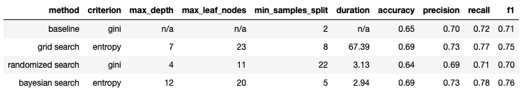
Table 1: Classification results from the 3 different hyperparameter tuning methods tested. Our baseline measurements are also included for comparison.
And now let’s tabulate the regression results:
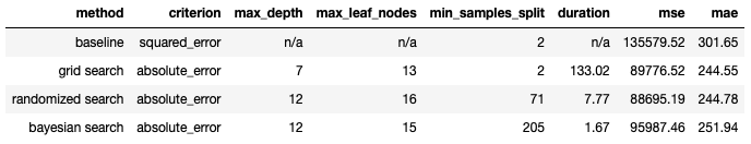
Table 2: Regression results from the 3 different hyperparameter tuning methods tested. Our baseline measurements are also included for comparison.
The tabulated results summarise the different methods used here to tune our models. The baseline indicates model performance using the default hyperparameter values.
For the classification results, we can see that both Grid Search & Bayesian Search yield comparable results. Both demonstrate an improvement over the baseline. The Randomised Search yields results that are very similar to the baseline.
In the regression case, both Grid Search & Randomised Search yield similar results. The Bayesian Search yields a model that performs worse compared to the other two methods. It should be noted that all 3 tuning methods produce models that are more performative than the baseline.
Two key things to note:
- There is a noticeable pattern in the duration times for all 3 methods attempted. Grid Search takes by far the longest time to compute, whereas Bayesian Search is the quickest.
- The performance obtained from the tuning methods will depend on the distributions used to define the parameter space. For Randomised Search & Bayesian Search, the number of samples extracted from the hyperparameter space will also influence the results. For Bayesian Search, the choice of prior will also be important.
I hope you enjoyed this article on how to tune hyperparameters in Decision Trees. Feel free to copy the code presented here into your own Python notebooks or scripts. Play with different settings and configurations of the tuners, to see if you can get better results for shorter computation times!
Related Posts
Hi I'm Michael Attard, a Data Scientist with a background in Astrophysics. I enjoy helping others on their journey to learn more about machine learning, and how it can be applied in industry.
Very interesting!… keep them coming.
[…] the setting of hyperparameters. We already explored hyperparameter tuning for Decision Trees in a previous article. Pre-Pruning is similar to hyperparameter tuning, except that we limit ourselves to only those […]