For classification problems, information gain in Decision Trees is measured using the Shannon Entropy. The amount of entropy can be calculated for any given node in the tree, along with its two child nodes. The difference between the amount of entropy in the parent node, and the weighted average of the entropies in the child nodes, yields the amount of information gain at that stage in the tree.
Table of Contents
What is the Shannon Entropy?
The Shannon Entropy is a quantity that measures the level of disorder in a system. Put in other words, the Shannon Entropy measures the level of uncertainty there is for the outcome of a given process. Let’s look at an illustrative example to gain some intuition on this. Consider the case of a set of circles with two possible types, red and blue. Now let us imagine that we obtain 3 different samples of circles from this set. These samples are depicted in Figure 1:
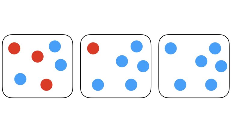
Figure 1: Three samples containing two possible classes of circles: red or blue. The amount of entropy in each sample is indicative of the level of disorder, and decreases as we look from left to right.
If we attempt to randomly pick one circle out of any of these three samples, what would we expect to get? From the left-most sample, we have a 50%-50% chance of getting a red or blue circle. Entropy is high here, since we are not very certain of the outcome. From the middle sample, there is a 5/6 chance of selecting a blue circle, and a 1/6 chance of getting a red one. Entropy has reduced, since we are fairly confident that a blue circle will be selected. The right-most sample is entirely composed of blue circles, yielding an entropy of zero. Picking a circle from this sample is guaranteed to yield a blue circle.
Let’s extend the above example, to a scenario where there are six possible classes of circles:
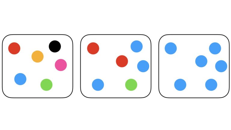
Figure 2: Three samples containing six possible classes of circles: red, blue, orange, pink, green, or black. Like in Figure 1, entropy decreases from left to right. However, because of the increased number of classes, the maximum possible entropy is larger in this example.
Like before, we can imagine having sampled the 6-class set three times. The hypothetical results of this sampling are illustrated in Figure 2.
Now what can we expect to get from randomly choosing one circle out of these samples? The left-most sample contains one circle from each class, so the chance of obtaining any one class is 1/6. Entropy is very high here, since there is a low expectation for any class in the set. Note that the entropy here is greater than in the two-class scenario.
Looking at the middle sample, we have a 50% chance of getting a blue circle, and 2/6 and 1/6 chances of getting red and green circles, respectively. Entropy has reduced in comparison to the left-most sample, yet we are still not certain of the outcome. Like in the 2-class example, the right-most sample is entirely composed of blue circles. As such, the entropy here is zero.
We can now define the Shannon Entropy mathematically:
H = -\sum_c p_c\log_2(p_c) (1)
where p_c is the probability of obtaining class c from a selection process. This quantity originates from information theory, and was defined by Claude Shannon in 1948. The units of H are bits. It is an appropriate function to measure the amount of “choice” involved in a selection, or the degree of uncertainty in an outcome.
The functional form of (1) is plotted in Figure 3 for data consisting of 2 and 6 classes:
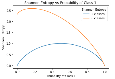
Figure 3: Functional form of the Shannon Entropy for the 2-class and 6-class cases, as a function of p_{c_1}. Note the left-hand side of the plot is computed with the maximum representation of all classes except c_1. In general, the more classes that are present, the larger the maximum entropy will be.
The Shannon Entropy is a downward concave function of p_c, that has a minimum of 0.0 and a maximum that depends on the number of classes in the data. For the 2-class case, we see the maximum reached is 1.0. On the other hand, for 6 classes a maximum entropy of 2.6 is attained.
Computing Information Gain in Decision Trees
Within Decision Tree classifiers, the Shannon Entropy can be used as a splitting criteria during training. This metric is used to determine how best to split the labeled data available at any given node. By “best”, I mean which split of the data will most reduce the entropy in the resulting two child nodes. The information gain resulting from the split is then given by:
\text{information gain} = H_{\text{parent}}-(w_1H_{\text{child 1}} + w_2H_{\text{child 2}}) (2)
where H_{\text{parent}} is the entropy in the parent node prior to the split, H_{\text{child 1}} and H_{\text{child 2}} are the entropies in the child nodes after the split, and w_1 and w_2 are proportional weights that sum to 1.0. Therefore, the goal at each node in the Decision Tree is to use the optimal splitting rule that will maximise the information gain. For more details on how Decision Trees are built during training, please refer to my article on the topic here.
Python Examples
In this section, we will work through the steps of computing information gain at individual nodes in a Decision Tree. Let’s start by importing the necessary Python packages:
import numpy as np
import pandas as pd
import seaborn as sn
import matplotlib.pyplot as plt
from sklearn.datasets import make_classification
from sklearn.model_selection import train_test_split
Our implementation of the Shannon Entropy now follows:
## function that implements the shannon entropy ##
def shannon_entropy(Data: np.array) -> float:
    """
    Function to compute the Shannon Entropy for a set of input data

    Inputs:
        Data => numpy 2D array of predictors & labels, where labels are assumed to be in the last column

    Outputs:
        H => Shannon Entropy value
    """
    #initialize the output
    H = 0
    #iterate through the unique classes
    for c in np.unique(Data[:,-1]):
        #compute p for the current c
        p = Data[Data[:,-1]==c].shape[0]/Data.shape[0]
        #compute term for the current c
        H -= p*np.log2(p)
    #return shannon entropy
    return(H)
Note that this function implements equation (1) for an input 2D numpy array.
The dataset will be generated using the make_classification functionality available from scikit-learn. We can generate a dataset of 100 samples with a total of 5 predictive features. Of these features, 2 will be informative for identifying the associated class. The label column will contain a total of 2 unique classes:
## create a classification dataset ##
X,y = make_classification(n_samples=100,
                          n_features=5,
                          n_informative=2,
                          n_classes=2,
                          weights=[0.4,0.6],
                          random_state=42)
We can visualise these data to get a better sense of what we have generated. First, let’s create a box plot of the predictive features:
## plot the distribution of the predictor features ##
plt.boxplot(X)
plt.xlabel('features')
plt.ylabel('values')
plt.title('Distributions in Features')
plt.xticks([1, 2, 3, 4, 5], ['x1', 'x2', 'x3', 'x4', 'x5'])
plt.show()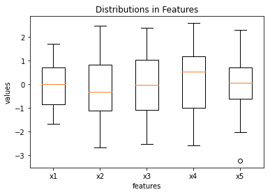
Three of the features (x1, x3, x5) possess medians that are approximately zero, the remaining two (x2 and x4) deviate from this somewhat. Outliers do not appear to be present in these data.
We can build a heat map of the predictive features, along with the label column. This can be used to reveal interesting correlations in the data:
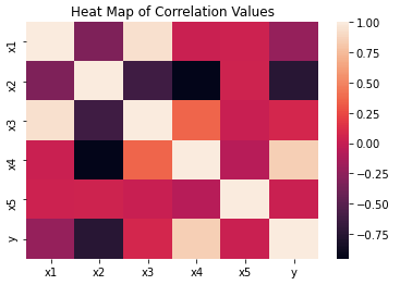
It’s clear from this figure that x2 and x4 are the most highly (anti-)correlated with the labels. We can therefore identify these features as the two informative predictors we specified in make_classification.
We can now work through the computation of information gain, by evaluating (2) on two different splits in these data.
Random Split of the Data
We can make a random split of the available data, into two parts of 60% and 40% of the original dataframe. Note that for the 2-class problem, the closer to H \approx 1.0 we get, the more disordered the labels are in each dataframe. Therefore the quality of the split will be poor, and we can expect little in terms of information gain. Conversely, the closer to H \approx 0.0, the more uniform the class labels are in each dataframe. The quality of the split will be better, and we can expect a larger information gain.
## make a random 60%, 40% split of the data ##
df1 = df.sample(frac=0.4, random_state=42)
df2 = pd.merge(df,df1,indicator=True,how='outer').query('_merge=="left_only"') \
                                                 .drop('_merge', axis=1)
Now we can compute H for the original dataframe, along with the dataframes resulting from the split. Afterwards, we can compute (2) to measure the information gain:
# compute the shannon entropy for df
shannon_entropy(df.values)
0.9709505944546686
# compute the shannon entropy for df1
shannon_entropy(df1.values)
0.934068055375491
# compute the shannon entropy for df2
shannon_entropy(df2.values)
0.9871377743721863
# compute information gain
shannon_entropy(df.values) - (0.4*shannon_entropy(df1.values) + 0.6*shannon_entropy(df2.values))
0.0050407076811603835
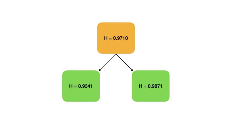
Figure 4: A visual representation of the random data split. The orange block represents the Shannon Entropy in the original data. Green blocks indicate the amount of entropy present after the split. Note that the entropies present after the split still remain close to \approx 1.0.
The information gain is positive, and as such this split has resulted in some increase in order. However, the amount of information gain (\approx 0.005) is minimal. This makes sense, since we do not expect to get the labels of each class isolated into individual dataframes from a random split.
Informed Split of the Data
We can try the same exercise as above, but this time we will attempt to make a more informed choice on how we make our split. Let’s base our split on the median of x4, which we know is one of our informative features:
## make a split based upon the median of x4 ##
med = df.x4.median()
df1 = df[df.x4 > med].copy()
df2 = df[df.x4 <= med].copy()

# compute the shannon entropy for df1
shannon_entropy(df1.values)
0.14144054254182067
# compute the shannon entropy for df2
shannon_entropy(df2.values)
0.7601675029619657
# compute information gain
shannon_entropy(df.values) - ((df1.shape[0]/df.shape[0])*shannon_entropy(df1.values) +
                              (df2.shape[0]/df.shape[0])*shannon_entropy(df2.values))
0.5201465717027753
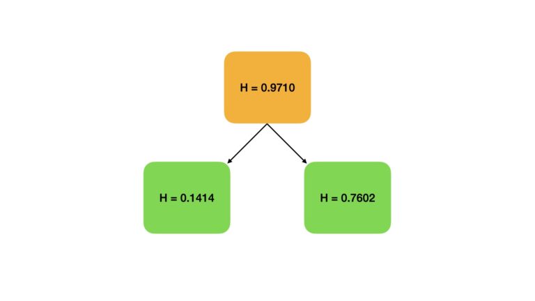
Figure 5: A visual representation of an informed split based upon feature x4. The orange block represents the Shannon Entropy in the original data. Green blocks indicate the amount of entropy present after the split. Note that the entropies present after the split show a significant reduction, indicating class labels have been isolated to a certain degree.
Although our “informed” splitting procedure is still rather crude, it has yielded a significant improvement over the random split. Our information gain now is \approx 0.52, which is just over half a bit of information, and approximately \times 100 the gain seen from the random split.
Final Remarks
In this post, you have seen how to determine information gain in Decision Trees. We have defined the Shannon Entropy, which is the fundamental metric required for this discussion. The exact mathematical form for computing information gain, between a parent and child nodes, has also been outlined. A couple of coding examples have been covered, which I hope made the concepts discussed here more understandable.
Within Decision Tree classifiers, the process of trying out different splitting criteria is automated during training. At each node in the tree, an input feature f, and split point s, are identified that maximises the information gain (2). In the informed split example discussed above, (f,s) are analogous to (x4,median(x4)). The parameters (f,s) are stored, and child nodes are created based upon the split of the training data they define.
Related Posts
Hi I'm Michael Attard, a Data Scientist with a background in Astrophysics. I enjoy helping others on their journey to learn more about machine learning, and how it can be applied in industry.
[…] an earlier article I introduced the Shannon Entropy, which is a measure of the level of disorder in a system. For discrete problems with class labels c […]