In this post, we will work through the implementation of a KNN Recommender System in Python. The model will be built up from scratch, and then tested on the MovieLens ml-25m dataset. The basic motivation, assumptions, and description behind the algorithm will also be covered.
Table of Contents
Motivation
In this post, we will work through the implementation of a KNN Recommender System in Python. Recommender systems are information retrieval algorithms, that are meant for situations where the end user has numerous different options to choose from. The intention is that the recommender will be able to filter through all the various options to arrive at the most relevant subset of choices. In this way, the end user gains convenience, and is able to save time, by solely focusing on only the most applicable options from the full suite of possibilities.
In general, recommender systems can be built using one of three approaches:
- Collaborative Filtering
- Content Based Filtering
- Hybrid (Collaborative Filtering + Content Based Filtering)
Here we will be using Collaborative Filtering, in conjunction with the K Nearest Neighbours (KNN) algorithm, to build a movie recommender for the MovieLens ml-25m dataset1. Collaborative filtering is a relatively simple and intuitive approach to the problem of recommendation, and has been widely used in industry. This technique was first developed as part of the Tapestry system by Xerox PARC, with their results being published in 1992.
Assumptions and Considerations
For our task here, we should keep in mind the following points:
- Since we will be making use of the KNN algorithm, the assumptions and considerations outlined in my previous article on this topic are also applicable here
- Collaborative filtering relies on users being active in our system. Tailored recommendations are not possible for users who have not yet interacted with the model, or not provided any information. For applications in production, workarounds should be considered. This is termed the cold-start problem
- Collaborative filtering also assumes that similar users can be grouped together solely based upon their past behaviour within the system (e.g. users who watch similar movies can be grouped together, etc). It ignores other meta information that might be relevant to the recommendation task (e.g. language, geographical location, movie directors, etc). There is also the implication that future choices can be predicted from recorded past behaviour
Description of the Collaborative Filtering KNN Algorithm
I will now describe collaborative filtering, through a simple illustrative example. Collaborative filtering works by using the past behaviour of users to build up a profile, from which like users can be grouped together. Items can then be recommended between like users, on the basis that their past behaviours should be a good indicator for future behaviour.
Let’s consider the case of movie recommendations. Imagine we have 4 users who have rated a series of movies belonging to 2 possible genres: dinosaurs or comedy. The ratings can be between 1.0 (very negative) to 5.0 (very positive). To keep things simple, let’s only consider the top 4 ratings for each user. The results are visualised below in Figure 1:
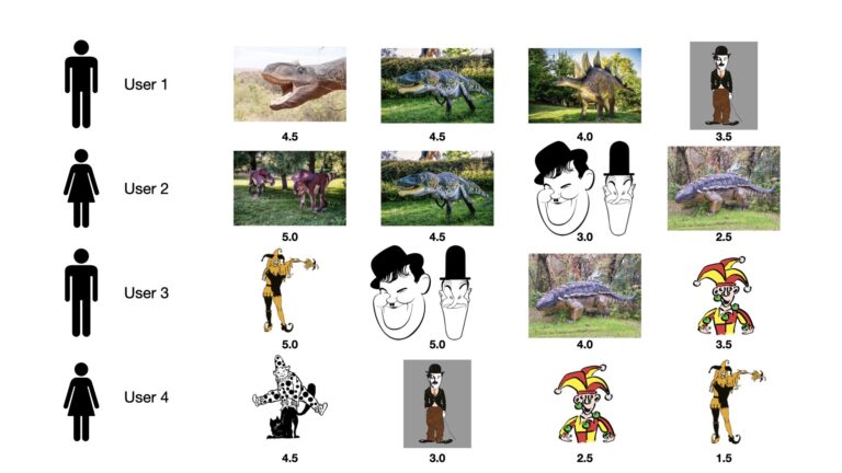
Figure 1: Top movie ratings for 4 users over a fictitious set of films. Each unique image represents a specific ‘movie’, which can belong to 1 of 2 possible genres: dinosaurs or comedy. The movies are listed horizontally in descending order, according to rating, for each user. The actual rating score is indicated below each image, and can range from 5.0 (very positive) to 1.0 (very negative).
The ratings illustrated in Figure 1 imply that users 1 and 2 have a preference for dinosaur movies, whereas users 3 and 4 prefer comedies. This inference is based on which types of movies tend to be the most highly rated per user, and the magnitude of the rating score itself. We can therefore make note that our set of users can be split into 2 groups of similar users: 1 & 2 and 3 & 4.
Recommendations can now be made through some straightforward logic: for each user we can recommend movies watched by their paired counterpart, but not yet viewed by that user. If we follow through with this line of reasoning, we can recommend movies to each user, as indicated in Figure 2:
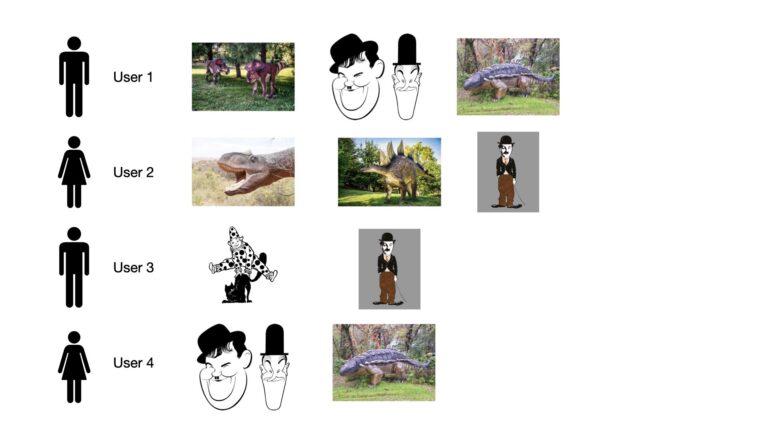
Figure 2: List of recommended movies per user. These recommendations are based upon what their similar user counterpart as viewed, but has not yet been watched by the user in question.
We can see the recommended movies per user in Figure 2 above. Note that users with a preference for dinosaurs (users 1 & 2) tend to get recommended other dinosaur movies. On the other hand, users who prefer comedies (users 3 & 4) tend to have other comedy movies recommended. This intuitively makes sense, and is what we would expect.
Above we glossed over how we can infer which users are most similar to each other. Let’s now discuss this in some more formal detail. One simple approach is to construct two column vectors per user: one for each genre. These vectors can be populated with the rating scores assigned to them by the respective user. Figure 3 depicts this setup:
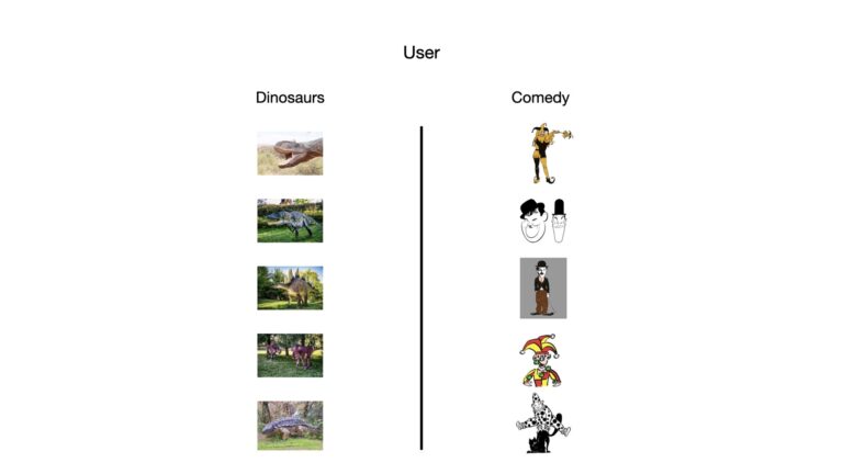
Figure 3: Pictorial depiction of a basic feature setup. Each user will have two columnar vectors, one containing ratings scores given to dinosaur movies, the other for comedies. The ratings in each vector will be ordered according to the images in this figure.
Following the scheme illustrated above, we can now create some basic features for each of our 4 users. Let’s show these now:
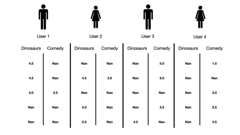
Figure 4: Depiction of rudimentary features for each user in our example. Rating scores assigned by the user to each movie populate the vectors. Entries filled with ‘Nan’ indicate movies that the user hasn’t watched yet.
The vectors in Figure 4 could form the basis for input features to a recommender model. Further processing would be needed to account for:
- missing values (Nan’s)
- combining the 2 genre-specific vectors, per user, into a single unique feature for the user
- any additional processing that might be desirable
After the processing is done, the resulting vectors form a matrix with columns for individual users, and rows for individual movies. It should be emphasised that the way this feature matrix is constructed will depend on the nature of the problem at hand, and the data that is available. However, the end result will typically be a matrix of item information (i.e. movies) versus users.
For the purposes of this article, we will make use of K-Nearest Neighbours to group users based upon their unique feature vectors. I covered this algorithm in detail in a previous post. We will exclusively use cosine similarity to achieve this, as this distance metric typically performs well for high dimensional data, and has a standard output ranging between (-1,+1). Consider two vectors \bold{A} = (a_1, a_2, … a_N) and \bold{B} = (b_1, b_2, … b_N), each of which have N components. The cosine similarity of these two vectors is given by:
\textrm{cosine} \: \textrm{similarity} = \frac{\sum_i^N{a_i b_i}}{ \sqrt{\sum_i^N a^2_i} \sqrt{\sum_i^N b^2_i}} (1)
If \bold{A} and \bold{B} are aligned, equation (1) will yield +1. If they are orthogonal, 0 will result, while if the vectors are opposite -1 will be the result. As such, the closer the cosine similarity is to +1, the more similar the two vectors are.
Implementation of a Collaborative Filtering KNN Recommender in Python
We can now work through the various steps needed to build our movie KNN recommender system. As mentioned earlier, the dataset we’ll be using is the MovieLens ml-25m dataset1. The feature engineering pipeline required was discussed in a previous post on pandas pipelines. This pipeline includes 3 stages, which are implemented below:
## pipeline stages ##
def prepare_ratings(dfRatings: pd.DataFrame) -> pd.DataFrame:
    """
    function to preprocess ratings dataframe

    Inputs:
        dfRatings -> dataframe containing ratings information

    Outputs:
        ratings dataframe without timestamp column
    """
    dfRatings.drop(['timestamp'],axis=1,inplace=True)
    return dfRatings

def prepare_tags(dfRatings: pd.DataFrame,
                 dfTags: pd.DataFrame,
                 dfGtags: pd.DataFrame,
                 dfGscores: pd.DataFrame,
                 threshold: float) -> pd.DataFrame:
    """
    function to execute preprocessing on the tags dataframes

    Inputs:
        dfRatings -> dataframe containing ratings information
        dfTags    -> dataframe containing tags information
        dfGtags   -> dataframe containing tag genome information
        dfGscores -> dataframe containing tag relevance information
        thresold  -> cutoff threshold based upon tag popularity

    Output:
        dataframe containing the prepared tags features merged to dfRatings
    """
    # drop timestamp column
    dfTags.drop(['timestamp'],axis=1,inplace=True)

    # set tags to lower case
    dfTags['tag'] = dfTags.tag.str.lower()
    dfGtags['tag'] = dfGtags.tag.str.lower()

    # join dfTags, dfGtags, & dfGscores
    dfTagScores = pd.merge(dfTags,dfGtags,on='tag')
    dfTagScores = pd.merge(dfTagScores,dfGscores,on=['movieId','tagId'])

    # extract usable tagId's based on cutoff threshold
    dfTagIds = dfTagScores[['userId','tagId']].copy()
    dfTagIds.drop_duplicates(inplace=True)
    dfTagIds['occurance'] = 1
    sTagIds = dfTagIds.groupby(by=['tagId'])['occurance'].sum().sort_values(ascending=False)
    tagIds = sTagIds[:threshold].index

    # OHE the tags, then multiply in the relevance
    sTags = dfTagScores[dfTagScores.tagId.isin(tagIds)].tag
    dfOHE = pd.get_dummies(sTags)
    dfTagsOHE = dfOHE.mul(dfTagScores.relevance,axis=0)

    # do final assembly of tags dataframe
    dfTags = pd.concat([dfTagScores[['userId','movieId','tagId']],dfTagsOHE],axis=1)

    # return merged results
    return pd.merge(dfRatings,dfTags,on=['userId','movieId'])

def prepare_movies(dfRatings: pd.DataFrame,
                   dfMovies: pd.DataFrame) -> pd.DataFrame:
    """
    function to execute preprocessing on the movies dataframe

    Inputs:
        dfRatings -> dataframe containing ratings information
        dfMovies  -> dataframe containing movies-genre information

    Output:
        dataframe containing the prepared movies-genre features merged to dfRatings
    """
    # helper function for use when creating genre features
    def flag_genre(row):
        applicable_genres = row['genres'].split('|')
        for genre in applicable_genres:
            row[genre] = 1
        return row

    # obtain the unique set of genres
    raw_genres = dfMovies.genres.unique()
    genres     = [g.split('|') for g in raw_genres]
    genres     = list(set(chain(*genres)))

    # create a set of binary features for each genre
    dfGenres = pd.DataFrame(0,columns=genres,index=np.arange(dfMovies.shape[0]))
    dfMovies = pd.concat([dfMovies, dfGenres], axis=1, join='inner')
    dfMovies = dfMovies.apply(flag_genre, axis=1)

    #drop irrelevant columns
    dfMovies.drop(['title','genres'],axis=1,inplace=True)

    # merge and multiply through the ratings score
    dfOut               = pd.merge(dfRatings,dfMovies,on='movieId')
    dfOut.loc[:,genres] = dfOut[genres].mul(dfOut.rating,axis=0)

    # return
    return dfOut
These three stages accomplish:
- prepare_ratings : function to prepare the ratings dataframe. This amounts to removing the timestamp column
- prepare_tags : function to generate features from three input tags dataframes, and join the result to the ratings dataframe. These features consist of relevance scores per user tag
- prepare_movies : function to build features from movie genre information. The features consist of user rating scores per genre
The features produced by these stages can then be used to identify similar users. This task will be done by an adapted version of the KNN class implemented in the previous article on K-Nearest Neighbours:
class KNN(object):
    """
    Class for KNN recommender system
    """

    def __init__(self, K : int = 3) -> None:
        """
        Initializer function for the class.
        Inputs:
            K      -> integer specifying number of neighbours to consider
        """
        # store/initialise input parameters
        self.K       = K
        self.dfXtrain = pd.DataFrame()

    def __del__(self) -> None:
        """
        Destructor function.
        """
        del self.K
        del self.dfXtrain

    def __cosine(self, sUser : pd.Series) -> pd.DataFrame:
        """
        Private function to compute the cosine similarity between point sUser and the training data dfXtrain
        Inputs:
            sUser -> pandas series data point of predictors to consider
        Outputs:
            dfCosine_s -> pandas dataframe of the computed similarities
        """
        # compute cosine similarity
        cosine_s = (np.dot(sUser,self.dfXtrain)/(np.linalg.norm(sUser)*np.linalg.norm(self.dfXtrain,axis=0)))
        # attach column headers
        dfCosine_s = pd.DataFrame(cosine_s.reshape((1,-1)),columns=self.dfXtrain.columns,index=['row'])
        # return
        return dfCosine_s

    def fit(self, dfX : pd.DataFrame) -> None:
        """
        Public training function for the class.
        It is assummed input dfX has been normalised, and columns represent distinct users.
        Inputs:
            dfX -> numpy array containing the predictor features
        """
        # store training data
        self.dfXtrain = dfX.copy()

    def predict(self, x_users : list) -> Dict:
        """
        Public prediction function for the class.
        Inputs:
            x_users -> list of userIds to make predictions for
        Outputs:
            dcOut -> dictionary containing the predicted K most similar users for each input userId
        """
        # ensure we have already trained the instance
        if self.dfXtrain.empty:
            raise Exception('Model is not trained. Call fit before calling predict.')
        # check for missing users (input userId's that aren't in the training data)
        missing_users = list(set(x_users) - set(self.dfXtrain.columns.values))
        if missing_users:
            print('The following input users are not present in the training data: {}\n\n'.format(missing_users))
        # work out valid users we can make recommendations for
        valid_users = list(set(x_users) - set(missing_users))
        print('Total number of input users to be analysed: {}'.format(len(valid_users)))
        # loop through each input user to identify the K most similar users in the training data
        dcRec = {}
        for user in valid_users:
            # extract user
            sUser = self.dfXtrain[user].copy()
            # compute cosine similarity
            dfCosine_s = self.__cosine(sUser)
            # obtain the K nearest neighbours
            dfCosine_s = dfCosine_s.sort_values(by='row',ascending=False,axis=1)
            y_pred = dfCosine_s.iloc[:,1:(self.K+1)].columns.tolist()
            # store the predictions
            dcRec[user] = y_pred
        # return results
        return dcRec

    def get_params(self, deep : bool = False) -> Dict:
        """
        Public function to return model parameters
        Inputs:
            deep -> boolean input parameter
        Outputs:
            Dict -> dictionary of stored class input parameters
        """
        return {'K':self.K}
The main updates to this implementation include:
- only one distance metric is supported: cosine similarity. This metric is maximised, so as to identify the most similar users to any particular user we wish to make recommendations for
- the predict function yields a dictionary containing lists of similar users for valid target users in x_users. Valid users are determined as those who have entries present in the training data. It is possible, for users having a minimal number of entries in the dataset, that all of their entries could be picked up during our sampling of the test set. This would result in the absence of these users from the training data, and thus makes tailored predictions impossible. The dictionary keys consist of the userIds of the valid users
Recommending movies then follows the logic outlined in the previous section of this article: for each user we can recommend movies watched by their most similar counterparts, but not yet viewed by that user. To measure how effective these recommendations are on a test set, I will make use of precision@k and recall@k. I will make use of the implementations outlined in my previous article on this topic:
def precision_at_k(df: pd.DataFrame, k: int=3, y_test: str='y_actual', y_pred: str='y_recommended') -> float:
    """
    Function to compute precision@k for an input boolean dataframe

    Inputs:
        df     -> pandas dataframe containing boolean columns y_test & y_pred
        k      -> integer number of items to consider
        y_test -> string name of column containing actual user input
        y_pred -> string name of column containing recommendation output

    Output:
        Floating-point number of precision value for k items
    """
    # check we have a valid entry for k
    if k <= 0:
        raise ValueError('Value of k should be greater than 1, read in as: {}'.format(k))
    # check y_test & y_pred columns are in df
    if y_test not in df.columns:
        raise ValueError('Input dataframe does not have a column named: {}'.format(y_test))
    if y_pred not in df.columns:
        raise ValueError('Input dataframe does not have a column named: {}'.format(y_pred))

    # extract the k rows
    dfK = df.head(k)
    # compute number of recommended items @k
    denominator = dfK[y_pred].sum()
    # compute number of recommended items that are relevant @k
    numerator = dfK[dfK[y_pred] & dfK[y_test]].shape[0]
    # return result
    if denominator > 0:
        return numerator/denominator
    else:
        return None

def recall_at_k(df: pd.DataFrame, k: int=3, y_test: str='y_actual', y_pred: str='y_recommended') -> float:
    """
    Function to compute recall@k for an input boolean dataframe

    Inputs:
        df     -> pandas dataframe containing boolean columns y_test & y_pred
        k      -> integer number of items to consider
        y_test -> string name of column containing actual user input
        y_pred -> string name of column containing recommendation output

    Output:
        Floating-point number of recall value for k items
    """
    # check we have a valid entry for k
    if k <= 0:
        raise ValueError('Value of k should be greater than 1, read in as: {}'.format(k))
    # check y_test & y_pred columns are in df
    if y_test not in df.columns:
        raise ValueError('Input dataframe does not have a column named: {}'.format(y_test))
    if y_pred not in df.columns:
        raise ValueError('Input dataframe does not have a column named: {}'.format(y_pred))

    # extract the k rows
    dfK = df.head(k)
    # compute number of all relevant items
    denominator = df[y_test].sum()
    # compute number of recommended items that are relevant @k
    numerator = dfK[dfK[y_pred] & dfK[y_test]].shape[0]
    # return result
    if denominator > 0:
        return numerator/denominator
    else:
        return None
KNN Recommender with the MovieLens ml-25m Dataset
We can now apply the functionality described in the previous section to the Movielens ml-25m dataset. I explored these data in my article on panadas pipelines, and as such I will not repeat that work here. Let’s start with the necessary imports, and then load in the data:
## imports ##
import numpy as np
import pandas as pd
from itertools import chain
import matplotlib.pyplot as plt
from typing import Dict

# load in data
dfRatings = pd.read_csv('./ml-25m/ratings.csv')
dfTags    = pd.read_csv('./ml-25m/tags.csv')
dfMovies  = pd.read_csv('./ml-25m/movies.csv')
dfLinks   = pd.read_csv('./ml-25m/links.csv')
dfGscores = pd.read_csv('./ml-25m/genome-scores.csv')
dfGtags   = pd.read_csv('./ml-25m/genome-tags.csv')
Okay, now let’s set a threshold value for our process_tags stage in our pipeline. Afterwards we can run preprocessing on the raw data:
# set cutoff threshold
threshold = 200

# construct a pipeline to carry out the preprocessing work outlined previously
dfPrepared = dfRatings.pipe(prepare_ratings) \
                      .pipe(prepare_tags,dfTags=dfTags,dfGtags=dfGtags,dfGscores=dfGscores,threshold=threshold) \
                      .pipe(prepare_movies,dfMovies=dfMovies)
The dataframe dfPrepared contains our combined, processed data. At this point, we can now split the data into train and test sets. I will select out 5% of the userId’s to form the test set:
# sample 5% of the user movie ratings
dfSelected = dfPrepared[['userId','movieId']].drop_duplicates().sample(frac=0.05,random_state=42).copy()
dfTest = pd.merge(dfPrepared,dfSelected,on=['userId','movieId'],how='inner')

# remove the test set to form a training set
dfTrainRaw = dfPrepared.drop(dfSelected.index.values).copy()
dfTrain = dfTrainRaw.copy()
User profiles can now be built using the training data. I’ll remove irrelevant columns, group over the userId’s and sum the entries, and then normalise the result:
# drop irrelevant columns
dfTrain.drop(['movieId','tagId','rating'],axis=1,inplace=True)

# groupby userId and sum
dfTrain = dfTrain.groupby(by=['userId']).sum()

# transpose the dataframe
dfTrain = dfTrain.transpose()

# normalise each user profile
dfTrain = (dfTrain-dfTrain.mean())/dfTrain.std()

# view the results
dfTrain.head(5)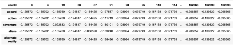
Great, we now have a dataframe where each column represents a unique userId, while each row is a different feature value. Let’s fit an instance of the KNN class on these data, and then obtain the most similar users for each userId in our test set (where possible):
# create a KNN instance with K = 10
recommender = KNN(K=10)

# fit the recommender instance
recommender.fit(dfTrain)

# obtain predictions
dcRec = recommender.predict(dfTest.userId.unique())
The following input users are not present in the training data: [6145, 30727, 98316, 66075, 153118, 111139, 51763, 76342, 132152, 158265, 28226, 34884, 134728, 152136, 109643, 138318, 102479, 99408, 73302, 108636, 56925, 19049, 69227, 73843, 20600, 36472, 127610, 14457, 53372, 60540, 82563, 145540, 104069, 132239, 63124, 108181, 8343, 111259, 136875, 160430, 109743, 46264, 14521, 9402, 58566, 131783, 47815, 17097, 95946, 84683, 32456, 110287, 58580, 106202, 66269, 40672, 66786, 7907, 68326, 83696, 2806, 25847, 113400, 28927, 30469, 79626, 67862, 39704, 66334, 126238, 15138, 10033, 129850, 121663, 73035, 137038, 44888, 126306, 152932, 20837, 39275, 127854, 123248, 34675, 127859, 136566, 55670, 58251, 71568, 31122, 27540, 54679, 114588, 105373, 37793, 141218, 94626, 100773, 1447, 18865, 118708, 56759, 144319, 137667, 107976, 24538, 11228, 85469, 7644, 141793, 65506, 161269, 81403, 123903] Total number of input users to be analysed: 2581
Listed above are the users we can’t make recommendations for, because their userId’s are not present in the training data. Despite this, we still have adequate data to test 2581 users. Let’s now make recommendations for each of these users, and then measure how effective our recommender is on the results. Since we will be using precision@k and recall@k metrics, we will need to convert the ratings into a binary relevant/non-relevant value. In addition we’ll need to set the k parameter. Let’s set the threshold parameter to 3.0, such that all ratings above this value are determined to be ‘relevant’, whereas anything equal to or below is ‘non-relevant’. I will also set k = 5, such that we’ll only consider five movies per user in our evaluation.
# select out the required columns from the raw training dataframe
dfTrainRaw = dfTrainRaw[['userId','movieId','rating']].drop_duplicates()

# set threshold for relevant/non-relevant movies, k for metrics, and initialise metrics lists
threshold = 3.0
k = 5
pre_at_k = []
rec_at_k = []

# loop through our test set results and evaluate recommendations
for userId in dcRec.keys():

    # get movies already watched
    movies_already_watched = dfTrainRaw[dfTrainRaw.userId == userId].movieId.unique()

    # collect all movies watched by the K similar users, and not already watched by userId
    dfSim = dfTrainRaw[ (~dfTrainRaw.movieId.isin(movies_already_watched)) &
                        (dfTrainRaw.userId.isin(dcRec[userId])) ].copy()

    # group on movieId, and then compute the mean rating
    dfRatings = dfSim.groupby(by='movieId')['rating'].mean().reset_index()
    dfRatings.columns = ['movieId','predicted_rating']

    # select out entries in the test set that correspond to our user
    dfTestUser = dfTest.loc[dfTest.userId == userId,['movieId','rating']].copy()
    dfTestUser.columns = ['movieId','actual_rating']

    # merge the user entries with the recommended movies
    dfResults = pd.merge(dfRatings,dfTestUser,on=['movieId'],how='inner').drop(['movieId'],axis=1)

    # convert results into boolean dataframe
    dfResults = dfResults > threshold

    # compute precision@k & recall@k
    patk = precision_at_k(dfResults,k=k,y_test='actual_rating',y_pred='predicted_rating')
    ratk = recall_at_k(dfResults,k=k,y_test='actual_rating',y_pred='predicted_rating')
    pre_at_k.append(patk)
    rec_at_k.append(ratk)
It is possible that our results arrays, pre_at_k and rec_at_k, contain missing values. The functions precision_at_k and recall_at_k will return None if the computation cannot be done. Let’s remove the None entries, and then summarise our findings:
# remove missing values
pre_at_k = np.array([i for i in pre_at_k if i is not None])
rec_at_k = np.array([i for i in rec_at_k if i is not None])

# compute statistics on our results
print('Precision@k mean: {0}, median: {1}, and standard deviation: {2}'.format(np.mean(pre_at_k),
                                                                               np.median(pre_at_k),
                                                                               np.std(pre_at_k)))
print('Recall@k mean: {0}, median: {1}, and standard deviation: {2}'.format(np.mean(rec_at_k),
                                                                            np.median(rec_at_k),
                                                                            np.std(rec_at_k)))
Precision@k mean: 0.8240777338603426, median: 1.0, and standard deviation: 0.35613771881889705 Recall@k mean: 0.8575273587695948, median: 1.0, and standard deviation: 0.31836093173585117
# plot the results
plt.hist(pre_at_k,alpha=0.5,edgecolor='black',label='precision@k',color='red')
plt.hist(rec_at_k,alpha=0.5,edgecolor='black',label='recall@k',color='yellow')
plt.title('Distribution of Precision@k and Recall@k for k=5')
plt.xlabel('score')
plt.ylabel('frequency')
plt.legend()
plt.show()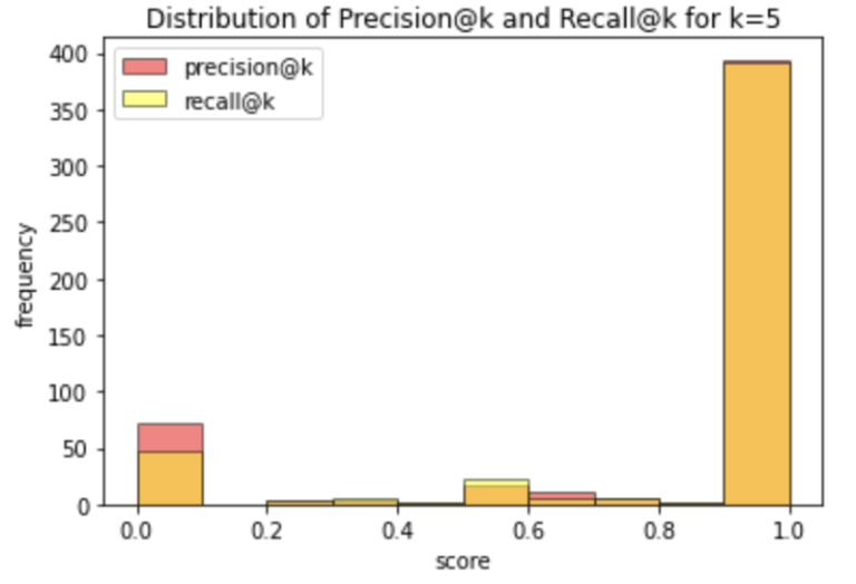
These results are quite encouraging: the mean and median results show that the top k=5 movie recommendations capture the clear majority of relevant movies in the test set. This conclusion is also supported by the histogram plot illustrating the distribution of results over the individual users.
Note that there are ways we can try to improve the model. One point that could be tried is to enhance how the ratings dataframe dfRatings is built from the output of the KNN instance. Here I computed the mean rating over the k most similar users. This does not take into account the relative degree of similarity these users have to the intended target user. You could try to extract the cosine similarity scores from the KNN instance, and use this to compute a weighted mean rating instead.
Final Remarks
In this article you have learned:
- What is Collaborative Filtering, and how it can be combined with K-Nearest Neighbours to build a recommender system
- The assumptions and considerations that need to be kept in mind when using a KNN recommender
- How to implement a KNN recommender in Python from scratch, and apply it to the MoveLens ml-25m dataset
I hope you enjoyed this article, and gained some value from it. If you would like to take a closer look at the code presented here, please take a look at my GitHub. If you have any questions or suggestions, please feel free to add a comment below. Your input is greatly appreciated.
Related Posts
References
- F. Maxwell Harper and Joseph A. Konstan. 2015. The MovieLens Datasets: History and Context. ACM Transactions on Interactive Intelligent Systems (TiiS) 5, 4: 19:1–19:19. https://doi.org/10.1145/2827872
Hi I'm Michael Attard, a Data Scientist with a background in Astrophysics. I enjoy helping others on their journey to learn more about machine learning, and how it can be applied in industry.
[…] to illustrate the concepts discussed. We can begin by considering a simple example involving movie recommendations. Imagine we have a pandas dataframe containing actual user movie ratings (y_actual), along with […]