Implement Gradient Boosting Regression in Python from Scratch

In this post, we will implement the Gradient Boosting Regression algorithm in Python. This is a powerful supervised machine learning model, and popularly used for prediction tasks. To gain a deep insight into how this algorithm works, the model will be built up from scratch, and subsequently verified against the expected behaviour.

Table of Contents

Motivation for Gradient Boosting Regression in Python

In the previous post, we covered how Gradient Boosting works, and outlined the general algorithm for this ensemble technique. Gradient Boosting was initially developed by Friedman 2001, and the general algorithm is referred to as Algorithm 1: Gradient_Boost, in that paper. Furthermore, we also discussed how to develop a practical Gradient Boosting procedure, based upon the absolute difference loss function, and Decision Tree weak learners. In this article, we will work through an implementation of this algorithm, named Algorithm 3: LAD_TreeBoost in Friedman 2001.

We will implement this algorithm in Python, as this is the most popular programming language for machine learning applications. My hope here is that by working through an implementation of this algorithm, and testing our code against different regression models available from scikit-learn, we can gain a deeper intuition for how these powerful algorithm work.

Brief Review of the LAD_TreeBoost Algorithm

Friedman’s 2001 paper describes a number of different applications of the Gradient_Boost algorithm. LAD_TreeBoost is one such application, and is considered to be a highly robust implementation of Gradient Boosting. For a more detailed description of these algorithms, please see my previous post.

Here, we defined an ensemble with $m = 1..M$ weak learners. We have defined our weak learners as regression Decision Trees, with $j=1..J$ terminal nodes that correspond to $R_{jm}$ terminal regions. Our loss has been chosen to be the absolute difference function.

Our data will consist of predictors $\bold{X}$ and targets $\bold{y}$ . We will index through each unique sample in the data with $n = 1..N$ .

$\bold{X} = \begin{bmatrix} \bold{x}_1 \\ \bold{x}_2 \\ . \\ . \\ \bold{x}_n \\ . \\ \bold{x}_N \end{bmatrix}$ , $\bold{y} = \begin{bmatrix} y_1 \\ y_2 \\ . \\ . \\ y_n \\ . \\ y_N \end{bmatrix}$ , where $\bold{x}_n \in R^{d}$ , $y_n \in R$

Note $\bold{x}_n$ are the rows of matrix $\bold{X}$ , and contain $d$ features. Similarly, $y_n$ are the scalar values of the column vector $\bold{y}$ .

Let’s now define the algorithm for LAD_TreeBoost:

Algorithm 3: LAD_TreeBoost

The training procedure is as follows:

$E_0(\bold{x}) = median(\bold{y}) = E_0$
For $m=1$ to $M$ :
$g_n = sign(y_n – E_{m-1}(\bold{x}_n))$ , for all $n=1..N$
Fit a $J$ terminal node Decision Tree to $\{ g_n,\bold{x}_n \}_1^N$ , and obtain the set of terminal regions $\{ R_{jm} \}_1^J$
$\gamma_{jm} = median_{\bold{x}_n \in R_{jm}}(y_n – E_{m-1}(\bold{x}_n))$ , for all $j = 1..J$
$E_m(\bold{x}) = E_{m-1}(\bold{x}) + \sum_{j=1}^J \gamma_{jm}I(\bold{x} \in R_{jm})$

This procedure will yield the initial ensemble value $E_0$ , the sets of parameters $\{ R_{jm} \}$ and $\{ \gamma_{jm} \}$ , and the set of $M$ trained Decision Trees. Note that $g_n$ are the gradients (from which the name of the algorithm is derived) and $\gamma_{jm}$ are model weights. The identity matrix is represented by $I$ .

Predictions from this ensemble, on a set of input data $\bold{x}’$ , can then be obtained by:

Initialise the ensemble to $E_0$
For $m=1$ to $M$ :
$E_m(\bold{x}’) = E_{m-1}(\bold{x}’) + \sum_{j=1}^J \gamma_{jm}I(\bold{x}’ \in R_{jm})$
Return $E_M(\bold{x}’)$

Implement LAD_TreeBoost in Python

We are now ready to implement Gradient Boosting regression in Python. I will encapsulate the logic described in the previous section into a single Python class. Let’s begin by importing the required packages to support our implementation:

import numpy as np
from typing import Dict, List, Tuple
from sklearn.tree import DecisionTreeRegressor

Our class definition, initialiser, and destructor functions are as follows:

## gradient boost tree regressor ##
class GradientBoostTreeRegressor(object):
    #initialiser
    def __init__(self, n_elements : int = 100, max_depth : int = 1) -> None:
        self.max_depth     = max_depth
        self.n_elements    = n_elements
        self.f             = []
        self.regions       = []
        self.gammas        = []
        self.mean_loss     = []
        self.e0            = 0
        
    #destructor
    def __del__(self) -> None:
        del self.max_depth
        del self.n_elements
        del self.f
        del self.regions
        del self.gammas
        del self.mean_loss
        del self.e0

__init__(self, n_elements, max_depth) : This is the initialiser that is called when a class instance is created. Input arguments include n_elements, which defines the size $M$ of the ensemble, and max_depth, which defines the size of each constituent Decision Tree.
__del__(self) : This is the destructor function that is called whenever a class instance is deleted. All resources associated with the instance are cleaned up here.

Next, we can define a private function to compute the ensemble weights $\gamma_{jm}$ :

    #private function to group data points & compute gamma parameters
    def __compute_gammas(self, yp : np.array, y_train : np.array, e : np.array) -> Tuple[np.array,Dict]:
        #initialise global gamma array
        gamma_jm = np.zeros((y_train.shape[0]))
        #iterate through each unique predicted value/region
        regions = np.unique(yp)
        gamma   = {}
        for r in regions:
            #compute index for r
            idx = yp == r
            #isolate relevant data points
            e_r = e[idx]
            y_r = y_train[idx]
            #compute the optimal gamma parameters for region r
            gamma_r = np.median(y_r - e_r)
            #populate the global gamma array
            gamma_jm[idx] = gamma_r
            #set the unique region <-> gamma pairs
            gamma[r] = gamma_r
        #append the regions to internal storage
        self.regions.append(regions)
        #return
        return((gamma_jm,gamma))

__compute_gammas(self, yp, y_train, e) : Here we have a private function to compute the logic described in Step 5 of our training procedure. The inputs to this function include predictions yp from the $m$ ^th weak learner, the training labels y_train ( $y_n$ ), and the state of the ensemble e ( $E_{m-1}$ ). The output from this function is a tuple containing the model parameters $\gamma_{jm}$ . The first element in the tuple is a numpy array that is formatted already for the training update. The second element is a dictionary that will be stored internally, and can be used when generating predictions.

We’re ready to define our public training procedure for this class:

    #public function to train the ensemble
    def fit(self, X_train : np.array, y_train : np.array) -> None:
        #reset the internal class members
        self.f             = []
        self.regions       = []
        self.model_weights = []
        self.mean_loss     = []
        #initialise the ensemble & store initialisation
        e0      = np.median(y_train)
        self.e0 = np.copy(e0)
        e       = np.ones(y_train.shape[0]) * e0
        #loop through the specified number of iterations in the ensemble
        for _ in range(self.n_elements):
            #store mae loss
            self.mean_loss.append(np.mean(np.abs(y_train - e)))
            #compute the gradients of our loss function
            g = np.sign(y_train - e)
            #initialise a weak learner & train
            model = DecisionTreeRegressor(max_depth=self.max_depth)
            model.fit(X_train,g)
            #compute optimal gamma coefficients
            yp             = model.predict(X_train)
            gamma_jm,gamma = self.__compute_gammas(yp,y_train,e)
            #update the ensemble
            e += gamma_jm
            #store trained ensemble elements
            self.f.append(model)
            self.gammas.append(gamma)

fit(self, X_train, y_train) : This public function takes in a matrix of predictors X_train ( $\bold{X}$ ) and their associated labels y_train ( $\bold{y}$ ). Within this function, Steps 1 through 6 of our training procedure are executed. The initial ensemble value $E_0$ , the trained weak learners (effectively $R_{jm}$ ), and the weights $\gamma_{jm}$ , are all stored internally.

Finally, let’s now define the remaining member functions for this class:

    #public function to generate predictions
    def predict(self, X_test : np.array) -> np.array:
        #initialise predictions
        y_pred = np.ones(X_test.shape[0]) * np.copy(self.e0)
        #cycle through each element in the ensemble
        for model,gamma,regions in zip(self.f,self.gammas,self.regions):
            #produce predictions using model
            y = model.predict(X_test)
            #cycle through each unique leaf node for model m
            for r in regions:
                #updates for region r
                idx = y == r
                y_pred[idx] += gamma[r] 
        #return predictions
        return(y_pred)
           
    #public function to return mean training loss
    def get_loss(self) -> List:
        return(self.mean_loss)
 
    #public function to return model parameters
    def get_params(self, deep : bool = False) -> Dict:
        return {'n_elements':self.n_elements,
                'max_depth':self.max_depth}

predict(self, X_test) : A public function that is used to produce predictions on unseen data X_test ( $\bold{x}’$ ). The predictions procedure, from the previous section, is run here.
get_loss(self) : Returns the mean absolute error loss, recorded at each iteration during training.
get_params(self, deep) : This is a public function to return the input arguments when an instance of this class is created. This function is required when using GradientBoostTreeRegressor instances in scikit-learn functions.

Testing Performance

We are now in a position to test our implementation of Gradient Boosting regression in Python. The data we will use here is the Diabetes Dataset available through scikit-learn. As I have already explored these data in my article on Adaboost regression, I will not repeat that analysis here. Let’s start by importing all the necessary packages to support our Gradient Boost implementation, and to conduct the analysis. Furthermore, we can load in the data:

## imports ##
import numpy as np
import pandas as pd
from typing import Dict, List, Tuple
import matplotlib.pyplot as plt
from sklearn.datasets import load_diabetes
from sklearn.model_selection import cross_validate
from sklearn.tree import DecisionTreeRegressor
from sklearn.metrics import mean_squared_error,mean_absolute_error,make_scorer
from sklearn.ensemble import RandomForestRegressor, AdaBoostRegressor

## load regression dataset ##
dfX,sy = load_diabetes(return_X_y=True,as_frame=True)

Note: rerunning the cells below will show some fluctuation in the results.

Investigate Training Loss

Here I want to look at how the training loss evolves as Decision Trees are added to the ensemble. In addition, I want to see what affect increasing the maximum depth, of the aforementioned Decision Trees, will have. The loss function displayed is the mean absolute error $\sum_i^N abs(y^{pred}_i – y^{true}_i)$ , at each iteration during training.

Now I will declare an instance of our custom Gradient Boost tree regressor for a series of max_depth values. Following each declaration, I will train the model on the raw data features, since Decision Trees typically require little in the way of preparatory feature engineering:

## train the gradient boost regressor with default max_depth ##
rgr = GradientBoostTreeRegressor(n_elements=100)
rgr.fit(dfX.values,sy.values)
## collect loss ##
loss1 = rgr.get_loss()

## train the gradient boost regressor with max_depth = 2 ##
rgr = GradientBoostTreeRegressor(n_elements=100, max_depth=2)
rgr.fit(dfX.values,sy.values)
## collect loss ##
loss2 = rgr.get_loss()

## train the gradient boost regressor with max_depth = 3 ##
rgr = GradientBoostTreeRegressor(n_elements=100, max_depth=3)
rgr.fit(dfX.values,sy.values)
## collect loss ##
loss3 = rgr.get_loss()

## train the gradient boost regressor with max_depth = 4 ##
rgr = GradientBoostTreeRegressor(n_elements=100, max_depth=4)
rgr.fit(dfX.values,sy.values)
## collect loss ##
loss4 = rgr.get_loss()

A plot of the collected loss functions nicely illustrates the results:

## plot different training losses ##
plt.plot(loss1,label='max_depth=1')
plt.plot(loss2,label='max_depth=2')
plt.plot(loss3,label='max_depth=3')
plt.plot(loss4,label='max_depth=4')
plt.title('Training Loss by Boosting Iteration')
plt.xlabel('Number of Component Trees')
plt.ylabel('MAE Loss')
plt.legend()
plt.show()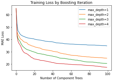

It is apparent that each model starts with a large loss value, which then declines rapidly before flattening out. It isn’t too surprising to see that ensembles with deeper trees achieve lower training losses. These models are expressive enough such that the data can be more accurately modelled, earlier in the boosting sequence. At the same time, the boosting procedure tackles any bias present.

Cross-Validation Analysis

Here I will use 10-fold cross-validation to measure the performance of the Gradient Boost regressor. I will set the maximum ensemble size to 20, and use a maximum depth of 1:

## define the scoring metrics ##
scoring_metrics = {'mse' : make_scorer(mean_squared_error), 
                   'mae': make_scorer(mean_absolute_error)}
                   
## perform cross-validation for n_elements = 20 & max_depth=1 ##
#define the model
rgr = GradientBoostTreeRegressor(n_elements=20,max_depth=1)
#cross validate
dcScores = cross_validate(rgr,dfX.values,sy.values,cv=10,scoring=scoring_metrics)
#report results
print('Mean MSE: %.2f' % np.mean(dcScores['test_mse']))
print('Mean MAE: %.2f' % np.mean(dcScores['test_mae']))

Mean MSE: 3548.21
Mean MAE: 46.56

We can compare these results with the Gradient Boost regressor available from scikit-learn:

from sklearn.ensemble import GradientBoostingRegressor

## perform cross-validation for n_estimators = 20 & max_depth=1 ##
#define the model
rgr = GradientBoostingRegressor(n_estimators=20,max_depth=1,loss='lad',learning_rate=1.0)
#cross validate
dcScores = cross_validate(rgr,dfX.values,sy.values,cv=10,scoring=scoring_metrics)
#report results
print('Mean MSE: %.2f' % np.mean(dcScores['test_mse']))
print('Mean MAE: %.2f' % np.mean(dcScores['test_mae']))

Mean MSE: 3549.82
Mean MAE: 46.65

Both Gradient Boost implementations perform at approximately the same level. Small differences between the two sets of results should be expected, due to the stochastic nature of the analysis.

Now let’s compare our results with a lone Decision Tree weak learner, a Random Forest Regressor with 20 constituent estimators, and an Adaboost Regressor also with 20 constituent estimators:

#cross validation for lone decision tree regressor of depth 1
dcScores = cross_validate(DecisionTreeRegressor(max_depth=1),dfX.values,sy.values,cv=10,scoring=scoring_metrics)
#report results
print('Mean MSE: %.2f' % np.mean(dcScores['test_mse']))
print('Mean MAE: %.2f' % np.mean(dcScores['test_mae']))

Mean MSE: 4751.55
Mean MAE: 56.68

## perform cross-validation for random forest regressor of n_estimators=20 and max_depth=1 ##
#define the model
rgr = RandomForestRegressor(n_estimators=20,max_depth=1)
#cross validate
dcScores = cross_validate(rgr,dfX.values,sy.values,cv=10,scoring=scoring_metrics)
#report results
print('Mean MSE: %.2f' % np.mean(dcScores['test_mse']))
print('Mean MAE: %.2f' % np.mean(dcScores['test_mae']))

Mean MSE: 3839.32
Mean MAE: 51.68

## perform cross-validation for linear loss & n_estimators=20 ##
#define the model
rgr = AdaBoostRegressor(base_estimator=DecisionTreeRegressor(max_depth=1), loss='linear', n_estimators=20)
#cross validate
dcScores = cross_validate(rgr,dfX.values,sy.values,cv=10,scoring=scoring_metrics)
#report results
print('Mean MSE: %.2f' % np.mean(dcScores['test_mse']))
print('Mean MAE: %.2f' % np.mean(dcScores['test_mae']))

Mean MSE: 3758.68
Mean MAE: 51.71

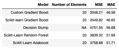
It is clear that the Gradient Boost Ensembles are the best performing models in this comparison. Adaboost takes second place, followed closely by the Random Forest. Unsurprisingly, the lone Decision Stump is the worst performing model attempted.

This simplistic analysis demonstrates the predictive potential of Gradient Boosting regression in Python. It is easy to understand why they have become popular for many applications and online competitions.

Final Remarks

In this article you have learned:

An overview of the LAD_TreeBoost Gradient Boosting algorithm
How to implement Gradient Boosting regression in Python from scratch
How our implementation of Gradient Boost compares against open-source, scikit-learn regression models

I hope you enjoyed this article, and gained some value from it. If you would like to take a closer look at the code presented here, please take a look at my GitHub. If you have any questions or suggestions, please feel free to add a comment below. Your input is greatly appreciated.

Cookie	Duration	Description
cookielawinfo-checkbox-analytics	11 months	This cookie is set by GDPR Cookie Consent plugin. The cookie is used to store the user consent for the cookies in the category "Analytics".
cookielawinfo-checkbox-functional	11 months	The cookie is set by GDPR cookie consent to record the user consent for the cookies in the category "Functional".
cookielawinfo-checkbox-necessary	11 months	This cookie is set by GDPR Cookie Consent plugin. The cookies is used to store the user consent for the cookies in the category "Necessary".
cookielawinfo-checkbox-others	11 months	This cookie is set by GDPR Cookie Consent plugin. The cookie is used to store the user consent for the cookies in the category "Other.
cookielawinfo-checkbox-performance	11 months	This cookie is set by GDPR Cookie Consent plugin. The cookie is used to store the user consent for the cookies in the category "Performance".
viewed_cookie_policy	11 months	The cookie is set by the GDPR Cookie Consent plugin and is used to store whether or not user has consented to the use of cookies. It does not store any personal data.