In general, Decision Trees are quite robust to the presence of outliers in the data. This is true for both training and prediction. However, care needs to be taken to ensure the Decision Tree has been adequately regularised. An overfitted Decision Tree will show sensitivity to outliers.
Table of Contents
Why are Decision Trees Robust to Outliers?
This feature of Decision Trees results from how these models are built. In a previous article I covered the CART Decision Tree algorithm, and how it can be implemented in Python from scratch. There are essentially two qualities that make Decision Trees robust to outliers:
- During training, the method to determine the optimal split point x_{f^*} and feature f^* makes use of an average calculated over sample of data. So long as this sample is sufficiently large, the effects of outliers will tend to be suppressed.
- Predictions from Decision Trees are based upon linear boundaries in data space. For example, is point x_f greater than or equal to x_{f^*}? The distance to the split point x_{f^*} is irrelevant.
Problems can arise in the event of overfitting. In this scenario, the sample sizes at each node can become small enough to effect the training procedure. As such, the values calculated for x_{f^*} and f^* can be significantly altered by the presence of outliers. This in turn will also have consequences for generating predictions. Note that in any event, it is standard practice to prevent overfitting of machine learning models!
Python Example
Let’s make the discussion outlined above more tangible with an example. We can test out the performance of the scikit-learn Decision Tree Regressor on two toy datasets: one with outliers and the other without. Furthermore, we can make one model with default hyperparameters (which will tend to overfit), and another with limits to how much the tree can grow during training.
Setup
We can start by importing the necessary packages, and then create a toy dataset to work with using scikit-learn’s make_regression:
# imports
import numpy as np
from sklearn.tree import DecisionTreeRegressor
from sklearn.model_selection import train_test_split
from sklearn.datasets import make_regression
import matplotlib.pyplot as plt
from sklearn.metrics import mean_absolute_error, mean_squared_error, median_absolute_error

# make a dataset
X,y = make_regression(n_samples=1000,
                      n_features=5,
                      n_informative=2,
                      n_targets=1,
                      bias=15.0,
                      noise=20.0,
                      random_state=42)
The dataset contains a total of 1000 samples, 5 predictive features, and 1 label. Of the predictive features, only 2 are informative. I have also introduced a bias term and noise component.
To get a better sense of what these data look like, let’s plot the predictive features together. We can also plot the distribution of the label as well.
# box plot of features
plt.boxplot(X)
plt.xlabel('features')
plt.ylabel('values')
plt.title('Distributions in Features')
plt.xticks([1, 2, 3, 4, 5], ['x1', 'x2', 'x3', 'x4', 'x5'])
plt.show()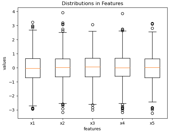
Figure 1: Boxplot of the predictive features in our toy dataset.
# histogram of label
plt.hist(y,bins=50)
plt.xlabel('y label')
plt.ylabel('frequency')
plt.title('Distribution in y Label')
plt.show()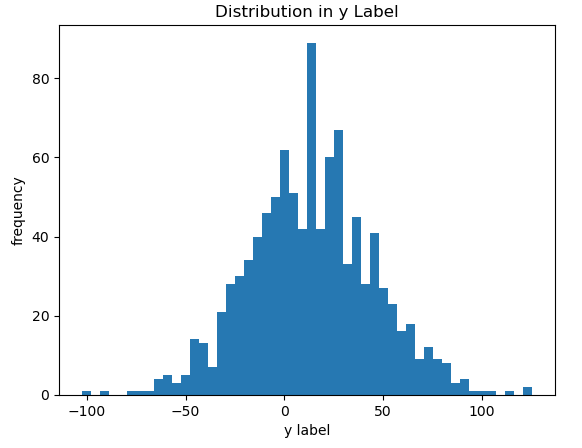
Figure 2: Histogram of the label values in the toy dataset.
Figure’s 1 & 2 show distributions that are consistent with the input parameters we provided to the make_regression function. Finally, we can perform a train-test split of the data:
# perform a train-test split
X_train, X_test, y_train, y_test = train_test_split(X, y, test_size=0.2, random_state=42)
Performance of Decision Tree Regressor without Outliers
Two different models will be tested: one with default hyperparameter values, and the other with a custom configuration. The default settings will allow the tree to grow during training as much as possible, and therefore provides no checks to overfitting. Our custom configuration will place limits on how much the tree can grow during training.
Let’s start with the default hyperparameters:
# fit the model & measure performance on the test set
rgr = DecisionTreeRegressor(random_state=42)
rgr.fit(X_train,y_train)
y_pred = rgr.predict(X_test)
print('mean absolute error: %.2f' % mean_absolute_error(y_test,y_pred))
print('mean squared error: %.2f' % mean_squared_error(y_test,y_pred))
print('median absolute error: %.2f' % median_absolute_error(y_test,y_pred))
mean absolute error: 22.90 mean squared error: 859.20 median absolute error: 17.25
And now we can try out the customised Decision Tree Regressor:
# fit the model & measure performance on the test set
rgr = DecisionTreeRegressor(max_depth=5,min_samples_split=50,random_state=42)
rgr.fit(X_train,y_train)
y_pred = rgr.predict(X_test)
print('mean absolute error: %.2f' % mean_absolute_error(y_test,y_pred))
print('mean squared error: %.2f' % mean_squared_error(y_test,y_pred))
print('median absolute error: %.2f' % median_absolute_error(y_test,y_pred))
mean absolute error: 15.98 mean squared error: 437.86 median absolute error: 12.63
In the customised model, we have set the max_depth and min_samples_split arguments to values that will greatly limit tree growth. And we can see the affects of this in the results: the customised model shows better overall performance in comparison to the default model. This is a clear indication that overfitting has occurred in the default model.
Note that since we’re working with a regression problem, I’m measuring performance here using the mean absolute error, mean squared error, and median absolute error metrics.
Introduce Outliers
We are now ready to introduce some pronounced outliers into our data. I will write code to replace 3% of the predictive feature samples with outliers. Afterwards, we can plot the predictive features to check the end result:
# percentage of outliers
percent_outliers = 0.03

# make copies
X_train_out = np.copy(X_train)
X_test_out  = np.copy(X_test)

# introduce outliers to train features
idx_rows = np.random.choice([i for i in range(X_train_out.shape[0])],
                            size=int(percent_outliers*X_train_out.shape[0]),
                            replace=False)
idx_cols = np.random.choice([i for i in range(X_train_out.shape[1])],
                            size=int(percent_outliers*X_train_out.shape[0]),
                            replace=True)
X_train_out[idx_rows,idx_cols] = X_train_out[idx_rows,idx_cols]*1e2

# introduce outliers to test features
idx_rows = np.random.choice([i for i in range(X_test_out.shape[0])],
                            size=int(percent_outliers*X_test_out.shape[0]),
                            replace=False)
idx_cols = np.random.choice([i for i in range(X_test_out.shape[1])],
                            size=int(percent_outliers*X_test_out.shape[0]),
                            replace=True)
X_test_out[idx_rows,idx_cols] = X_test_out[idx_rows,idx_cols]*1e2

# box plot of train features
plt.boxplot(X_train_out)
plt.xlabel('features')
plt.ylabel('values')
plt.title('Distributions in Train Features with Outliers')
plt.xticks([1, 2, 3, 4, 5], ['x1', 'x2', 'x3', 'x4', 'x5'])
plt.show()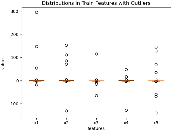
Figure 3: Predictive features for the training set, with outliers added.
# box plot of test features
plt.boxplot(X_test_out)
plt.xlabel('features')
plt.ylabel('values')
plt.title('Distributions in Test Features with Outliers')
plt.xticks([1, 2, 3, 4, 5], ['x1', 'x2', 'x3', 'x4', 'x5'])
plt.show()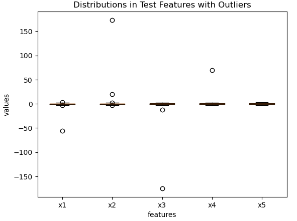
Figure 4: Predictive features for the test set, with outliers added.
Performance of Decision Tree Regressor with Outliers
Now let’s repeat the analysis done previously. But in this case with the new dataset, including outliers. First let’s try out a model with the default hyperparameters:
# fit the model & measure performance on the test set
rgr = DecisionTreeRegressor(random_state=42)
rgr.fit(X_train_out,y_train)
y_pred = rgr.predict(X_test_out)
print('mean absolute error: %.2f' % mean_absolute_error(y_test,y_pred))
print('mean squared error: %.2f' % mean_squared_error(y_test,y_pred))
print('median absolute error: %.2f' % median_absolute_error(y_test,y_pred))
mean absolute error: 23.85 mean squared error: 871.27 median absolute error: 21.30
And now the model with the custom hyperparameters:
# fit the model & measure performance on the test set
rgr = DecisionTreeRegressor(max_depth=5,min_samples_split=50,random_state=42)
rgr.fit(X_train_out,y_train)
y_pred = rgr.predict(X_test_out)
print('mean absolute error: %.2f' % mean_absolute_error(y_test,y_pred))
print('mean squared error: %.2f' % mean_squared_error(y_test,y_pred))
print('median absolute error: %.2f' % median_absolute_error(y_test,y_pred))
mean absolute error: 15.95 mean squared error: 433.73 median absolute error: 12.81
Like before, in the customised model we have set max_depth and min_samples_split to values that will limit tree growth during training. The results show the customised model has better overall performance in comparison to the default model. This is a clear indication that overfitting has occurred in the default model.
Results
We can tabulate the results obtained in the previous sections:
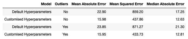
This table summarises our results. First, notice that the models with customised hyperparameters perform better than their default counterparts. This is evidence of overfitting in the default hyperparameter case. Second, the customised model yields results that are remarkably unaffected by outliers. On the other hand, the default model does show a small degradation in performance due to the presence of outliers. This highlights that while Decision Trees are generally robust to outliers, these models will become more sensitive to there presence if overfitting has occurred.
Final Remarks
In this article you have learned:
- Decision Trees are generally robust to outliers. However, as the Decision Tree becomes more overfitted to a training dataset, the model will become more affected by outliers.
- Why are Decision Trees robust to outliers.
- How we can test the robustness of the CART Decision Tree algorithm using a Python example.
I hope you enjoyed this article and gained value from it. If you have a question or comment regarding this article, please feel free to leave a comment below!
Related Posts
Hi I'm Michael Attard, a Data Scientist with a background in Astrophysics. I enjoy helping others on their journey to learn more about machine learning, and how it can be applied in industry.