In this post we will implement the Bootstrap Method, and use it to analyse a linear regression model. Through this exercise, we will understand how this technique works, and how you can apply the bootstrap method in Python from scratch.
Table of Contents
Note: for those who prefer video content, you can watch me work through the content in this article by scrolling to the bottom of this post.
Motivation to Implement the Bootstrap Method
A key question we can ask, regarding any modelling effort, is the uncertainty in our estimates. This applies both to the learned model parameters, as well as the resulting predictions obtained from a trained model. These uncertainty estimates could, for example, play an important role in choosing an optimal model for a given problem we want to solve. The bootstrap method provides a means by which these uncertainties can be quantified.
This article will be concerned with the non-parametric bootstrap method. In this case, no assumptions are made regarding the form of the underlying distribution from which our data was obtained.
The application of this technique is often used to calculate standard errors, confidence intervals, and to perform hypothesis testing on sample statistics. Prediction error can also be estimated. The bootstrap was first developed in 1979 by Bradley Efron1.
Bootstrap Method Assumptions and Considerations
The following assumptions will be required to develop and implement the bootstrap method:
- The data sample available accurately represents the true population of the data
- The variance of the true population is finite
Derivation of the Bootstrap Algorithm
We wish to use a Monte Carlo method by which uncertainties can be determined though the use of numerical methods. We will treat the available data as one of many possible samples that could have been obtained from the true underlying distribution.
Imagine a scenario where multiple samples are collected from a data source. For any given sample, a statistic computed on those data will vary between the different samples. This variation follows what is termed a sampling distribution.
The bootstrap method seeks to estimate this sampling distribution by continually resampling from the available data, with replacement. By “with replacement”, we mean that each data point in the available data can be resampled multiple times. Typically this resampling is done until the selected data is of equal size to the original sample. This process can be repeated multiple times to yield a set of resampled, bootstrapped samples.
The bootstrap method can therefore be outlined in the following 4 points:
- Ensure each data point in the original sample has equal probability of being selected
- Select a data point from the original sample for inclusion in the current bootstrap sample. This selection is done with replacement
- Repeat point 2. until the current bootstrap sample is the same size as the original sample
- Repeat points 2. & 3. until the required number of bootstrap samples are obtained
We can visualise this process below:
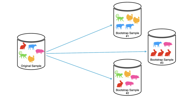
In this example, the original sample consists of 5 observations: the rabbit, cow, pig, turkey, and monkey. We run through the method outlined above to built three bootstrap samples. Note that each bootstrap sample consists of 5 observations, the same as the original sample. Also notice that in the boostrap samples some duplicates occur, and the same observation can be present in different bootstrap samples. This is a consequence of sampling with replacement.
In practice, anywhere from hundreds to thousands of bootstrap samples are normally generated during a statistical analysis.
Implement the Bootstrap Method in Python
We will start the worked example here by importing the required packages:
# imports
from typing import Tuple, Dict
import numpy as np
import matplotlib.pyplot as plt
import seaborn as sns
from sklearn.datasets import make_regression
from sklearn.linear_model import LinearRegression
from sklearn.model_selection import train_test_split
from sklearn.metrics import mean_absolute_error, mean_squared_error
Implement Bootstrap Functionality
Now I will define two functions that will help with our analysis:
def make_bootstraps(data: np.array, n_bootstraps: int=100) -> Dict[str, Dict[str, np.array]]:
    """
    Function to generate bootstrapped samples

    Inputs:
        data         -> array of input data
        n_bootstraps -> integer number of bootstraps to produce

    Outputs:
        {'boot_n': {'boot': np.array, 'test': np.array}} -> dictionary of dictionaries containing
                                                            the bootstrap samples & out-of-bag test sets
    """

    # initialize output dictionary, unique value count, sample size, & list of indices
    dc       = {}
    n_unival = 0
    sample_size = data.shape[0]
    idx = [i for i in range(sample_size)]
    # loop through the required number of bootstraps
    for b in range(n_bootstraps):
        # obtain boostrap samples with replacement
        sidx   = np.random.choice(idx,replace=True,size=sample_size)
        b_samp = data[sidx,:]
        # compute number of unique values contained in the bootstrap sample
        n_unival += len(set(sidx))
        # obtain out-of-bag samples for the current b
        oob_idx = list(set(idx) - set(sidx))
        t_samp = np.array([])
        if oob_idx:
            t_samp = data[oob_idx,:]
        # store results
        dc['boot_'+str(b)] = {'boot':b_samp,'test':t_samp}
    # state the mean number of unique values in the bootstraps
    print('Mean number of unique values in each bootstrap: {:.2f}'.format(n_unival/n_bootstraps))
    # return the bootstrap results
    return(dc)
The make_boostraps function takes in a numpy array data and generates the requested number of bootstrap samples set by the n_bootstraps argument. By default, this is set to 100. This function also calculates, and prints out, the mean number of unique data points contained in the bootstrap samples.
def prediction_error_by_training_size(train: np.array,
                                      test: np.array,
                                      train_sizes: list,
                                      iters: int=10) -> Tuple[list, list]:
    """
    Function to determine the relationship between model performance & training size

    Inputs:
        train       -> array containing training data
        test        -> array containing test data
        train_sizes -> list containing the integer number of samples to be used in the training set
        iters       -> number of repetitions to be done for each training size

    Outputs:
        (list,list) -> a tuple of two lists containing the average MAE and MSE errors for each train_sizes element
    """
    # initialize model & output lists
    lr    = LinearRegression()
    maes  = []
    mses  = []
    # get list of row indexes
    idx = [i for i in range(train.shape[0])]
    # loop over each training size
    for ts in train_sizes:
        # initialize error metrics
        mae = 0
        mse = 0
        # for each training size, repeat the calculation iters times
        for _ in range(iters):
            # obtain training samples without replacement
            sidx     = np.random.choice(idx,replace=False,size=ts)
            trainset = np.copy(train[sidx,:])
            # fit a linear regression model to the training set
            lr.fit(trainset[:,0].reshape(-1,1),trainset[:,1].reshape(-1,1))
            # generate predictions & calculate error metrics
            yp  = lr.predict(test[:,0].reshape(-1,1))
            mae += mean_absolute_error(test[:,1],yp)
            mse += mean_squared_error(test[:,1],yp)
        # store the mean error metrics over all repetitions
        maes.append(mae/iters)
        mses.append(mse/iters)
    # return error metrics
    return(maes,mses)
The function prediction_error_by_training_size computes the Mean Absolute Error and Mean Squared Error for predictions from a linear regression model. The MAE and MSE are given by:
MAE = \frac{1}{N}\sum_i^N|y_{i,pred}-y_{i,true}| (1)
MSE = \frac{1}{N}\sum_i^N(y_{i,pred}-y_{i,true})^2 (2)
where y_{pred} are the predicted values, y_{true} are the true values, and N is the total number of samples considered in the calculation. Note that the Root Mean Squared Error (RMSE) is simply the square root of the MSE. The lowest possible value is 0, indicating no deviation between the predicted and true values. The calculation of these error metrics is repeated over a number of different training sizes set by the list train_sizes. Since the selection of the training set is random, I repeat the calculations iters times and compute the mean for each training set size. With this function, we can analyse the effect of training size on model performance.
Data Exploration & Bias Check
We can now proceed to generate data to work with. I will make use of the make_regression function provided by scikit-learn:
# build a synthetic regression dataset
x,y,coef = make_regression(n_samples=5000,n_features=1,n_targets=1,coef=True,noise=5.0,bias=1.0,random_state=42)
Note that these data consist of 5000 samples with 1 dependent and 1 independent variables. The noise injected onto the dependent variable follows a normal distribution with a standard deviation of 5.0. The intercept is set to 1.0.
Let’s now plot these data:
# plot regression data
plt.scatter(x,y)
plt.xlabel('x-range')
plt.ylabel('y-range')
plt.title('Synethic Regression Data')
plt.show()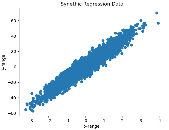
It is evident that we have highly dispersed data, which nonetheless have a positive slope.
We now need to consider the effects of bias and variance in our analysis. The aim of machine learning is to produce models that are able to generalise well beyond the training data used during fitting. Prediction error should ideally be due to noise in the data (i.e. the irreducible error).
Bias results from having a model that lacks the expressive ability to reproduce general trends seen in the data. This usually results from having insufficient training data, or from the choice of model.
On the other hand, Variance results from having a model that is too expressive, and as such is prone to becoming highly optimised on the training data. This results in a model that is too sensitive to noise present in the data, preventing it from generalising well.
For the current analysis, the variance problem is handled by the fact that we will be combining the results over many bootstrapped samples. This will have the effect of cancelling out the effects of variance over the aggregate. However, bias could be present due to the effect of the amount of unique data points available for training. If each bootstrap sample has an insufficient amount of unique data points to adequately train the model, then bias will be present in our results.
To check if bias will be a potential problem, let’s see how training set size effects model prediction accuracy. Let’s proceed to run the analysis:
# extract out a small test set to measure performance
xtrain,xtest,ytrain,ytest = train_test_split(x,y,test_size=0.1, random_state=42)
# define a set of training set sizes to choose from
train_size = [10,20,40,60,80,100,200,300,400]
# package the data
train = np.concatenate((xtrain,ytrain.reshape(-1,1)),axis=1)
test  = np.concatenate((xtest,ytest.reshape(-1,1)),axis=1)
# for each training set size, fit a model and calculate the error
maes,mses = prediction_error_by_training_size(train,test,train_size)
This code block performs a train-test split on the data, with 10% of the data allocated for testing. A set of 9 different training sizes are defined, and the data is packaged for use inside our function prediction_error_by_training_size. We can now plot the results:
# plot the error curves
plt.plot(train_size,maes)
plt.plot(train_size,np.sqrt(mses))
plt.title('Error Metric Dependence on Training Size')
plt.xlabel('Number of Unique Training Samples')
plt.ylabel('Error Metric Units')
plt.legend(['MAE','RMSE'])
plt.show()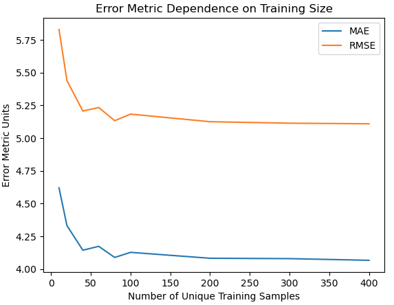
This plot shows that the linear regression model reaches optimal performance at a training set size of ~75 unique samples. As such, we should aim to have at least this number in each of our bootstrap samples.
Let’s now create 100 bootstrap samples from the complete dataset:
# package the data
data = np.concatenate((x,y.reshape(-1,1)),axis=1)
# generate bootstrap samples
dcBoot = make_bootstraps(data)
Mean number of unique values in each bootstrap: 3157.00
Note that the mean number of unique data points, in each bootstrap sample, is above 3000. This is well above the ~75 lower limit determined earlier. As such, we can conclude that bias shouldn’t be a major issue here in this analysis.
Bootstrap Analysis of Linear Regression
We now can iterate through each bootstrap sample, and fit a linear regression model to each sample. We can then collect the learned model parameters, as well as calculate the prediction errors using (1) and (2). The prediction errors are computed on the unique data points not selected in the current bootstrap sample. These are otherwise termed the out-of-bag samples.
# initialize storage variables & model
coefs = np.array([])
intrs = np.array([])
maes  = np.array([])
mses  = np.array([])
lr    = LinearRegression()
# loop through each bootstrap sample
for b in dcBoot:
    # fit a linear regression model to the current sample
    lr.fit(dcBoot[b]['boot'][:,0].reshape(-1, 1),dcBoot[b]['boot'][:,1].reshape(-1, 1))
    # store model parameters
    coefs = np.concatenate((coefs,lr.coef_.flatten()))
    intrs = np.concatenate((intrs,lr.intercept_.flatten()))
    # compute the predictions on the out-of-bag test set & compute metrics
    if dcBoot[b]['test'].size:
        yp  = lr.predict(dcBoot[b]['test'][:,0].reshape(-1, 1))
        mae = mean_absolute_error(dcBoot[b]['test'][:,1],yp)
        mse = mean_squared_error(dcBoot[b]['test'][:,1],yp)
        # store the error metrics
        maes = np.concatenate((maes,mae.flatten()))
        mses = np.concatenate((mses,mse.flatten()))
Let’s plot a histogram of the linear regression coefficient, along with some statistical information. Note that re-running this code can produce slightly different results. This is due to the random selection process built into the bootstrap method.
# plot histogram of regression coefficients
sns.displot(coefs, kde=True)
plt.title('Linear Regression Coefficient Data', fontsize=18)
plt.xlabel('Coefficients', fontsize=14)
plt.ylabel('Frequency', fontsize=14)
plt.show()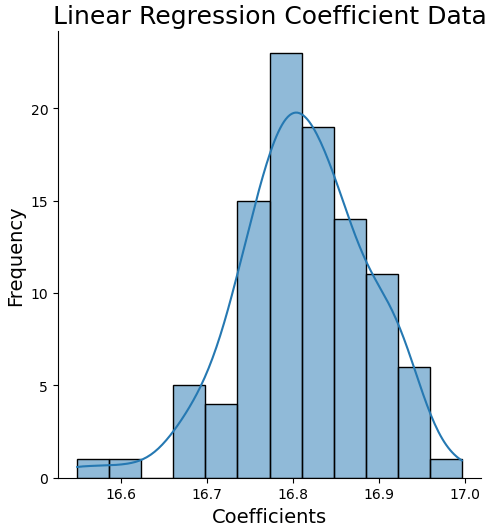
# compute statistics on model coefficient
print('Expected value: {:.2f}'.format(np.mean(coefs)))
print('Estimate Standard Error: {:.2f}'.format(np.std(coefs)/np.sqrt(coefs.shape[0])))
print('99% Confidence Interval for regression coefficient: {0:.2f} - {1:.2f}'.format(np.percentile(coefs,0.5),
                                                                                     np.percentile(coefs,99.5)))
Expected value: 16.81 Estimate Standard Error: 0.01 99% Confidence Interval for regression coefficient: 16.58 - 16.97
The true coefficient was obtained directly when calling make_regression:
# what is the true regression coefficient?
print('True regression coefficient: {:.2f}'.format(coef))
True regression coefficient: 16.82
The true value falls within the 99% confidence interval determined from our bootstrap samples, as well as within +/- 1 standard error about the expected value.
We can now do a similar analysis for the model intercept:
# plot histogram of regression intercepts
sns.displot(intrs, kde=True)
plt.title('Linear Regression Intercepts Data', fontsize=18)
plt.xlabel('Intercepts', fontsize=14)
plt.ylabel('Frequency', fontsize=14)
plt.show()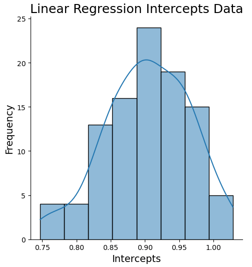
# compute statistics on model intercept
print('Expected value: {:.2f}'.format(np.mean(intrs)))
print('Estimate Standard Error: {:.2f}'.format(np.std(intrs)/np.sqrt(intrs.shape[0])))
print('99% Confidence Interval for regression intercept: {0:.2f} - {1:.2f}'.format(np.percentile(intrs,0.5),
                                                                                   np.percentile(intrs,99.5)))
Expected value: 0.90 Estimate Standard Error: 0.01 99% Confidence Interval for regression intercept: 0.75 - 1.03
The true intercept was set to 1.0. We can see that the true value falls within 99% confidence interval. However the range \{\text{expected value} – \text{standard error}, \text{expected value} + \text{standard error}\} does not cover the true intercept value. We can conclude that the intercept value we get with these data, from a linear regression fit, will tend to be underestimated.
Let’s now produce histogram plots of the prediction MAE and RMSE, along with their respective statistics:
# plot histogram of mae on predictions
sns.displot(maes, kde=True)
plt.title('Linear Regression Prediction MAE Results', fontsize=18)
plt.xlabel('MAE', fontsize=14)
plt.ylabel('Frequency', fontsize=14)
plt.show()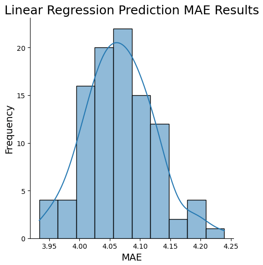
# compute statistics on MAE results
print('Expected value: {:.2f}'.format(np.mean(maes)))
print('Estimate Standard Error: {:.2f}'.format(np.std(maes)/np.sqrt(maes.shape[0])))
print('99% Confidence Interval for Prediction MAE results: {0:.2f} - {1:.2f}'.format(np.percentile(maes,0.5),
                                                                                     np.percentile(maes,99.5)))
Expected value: 4.07 Estimate Standard Error: 0.01 99% Confidence Interval for Prediction MAE results: 3.94 - 4.22
# plot histogram of rmse on predictions
sns.displot(np.sqrt(mses), kde=True)
plt.title('Linear Regression Prediction RMSE Results', fontsize=18)
plt.xlabel('RMSE', fontsize=14)
plt.ylabel('Frequency', fontsize=14)
plt.show()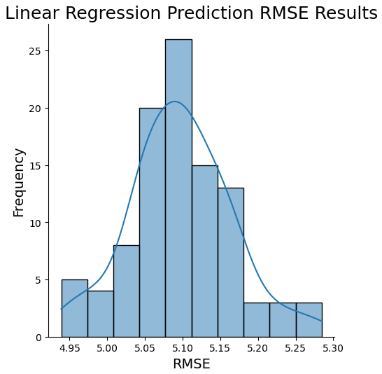
# compute statistics on RMSE results
rmse = np.sqrt(mses)
print('Expected value: {:.2f}'.format(np.mean(rmse)))
print('Estimate Standard Error: {:.2f}'.format(np.std(rmse)/np.sqrt(rmse.shape[0])))
print('99% Confidence Interval for Prediction RMSE results: {0:.2f} - {1:.2f}'.format(np.percentile(rmse,0.5),
                                                                                      np.percentile(rmse,99.5)))
Expected value: 5.10 Estimate Standard Error: 0.01 99% Confidence Interval for Prediction RMSE results: 4.94 - 5.28
The histograms above, along with the associated 99% confidence intervals, gives us a sense for the possible range in prediction error from this model. Note that the injected noise level of 5.0 falls nicely within the 99% confidence interval for the RMSE. If we look at the bias-variance breakdown of the MSE, we can see that this is expected:
MSE = Bias^2 + Variance + \sigma^2 (3)
In our case, we know that our data originates from a linear relationship between 1 independent variable and 1 dependent variable, with some injected noise (\sigma). As we have a sufficient number of samples in our dataset (and also in each bootstrap sample), it is fair to conclude that the effect of bias and variance should be minimal in our analysis. Therefore MSE \approx \sigma^2 or RMSE \approx \sigma.
Finally, we can produce a plot of the data with the expected linear regression fit. In addition, we can plot bounds around which the true linear relationship likely lies. These bounds will be based off of the RMSE estimates we calculated earlier:
# plot the model against the dataset
xp = np.linspace(min(x),max(x),100)
plt.figure(figsize=(15,10))
plt.plot(xp,np.mean(coef)*xp+np.mean(intrs),color='r')
plt.scatter(x=data[:,0],y=data[:,1],color='b')
plt.plot(xp,np.mean(coef)*xp+np.mean(intrs)+np.mean(np.sqrt(mses)),'-.g',linewidth=2)
plt.plot(xp,np.mean(coef)*xp+np.mean(intrs)-np.mean(np.sqrt(mses)),'-.m',linewidth=2)
plt.title('Linear Regression Fit to Generated Data', fontsize=18)
plt.xlabel('X', fontsize=14)
plt.ylabel('Y', fontsize=14)
plt.legend(['Model','Data','Model+RMSE','Model-RMSE'],loc='lower right')
plt.show()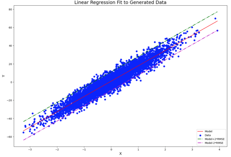
Note that the RMSE used in this plot is the expected value. Since the RMSE approximates the gaussian noise, I multiply by a factor of 2 to have upper/lower bounds that account for ~95% of the spread in the data.
Final Remarks & Video
In this article you’ve learned:
- The motivation behind the bootstrap method and when it was developed
- The methodology of the algorithm
- How to implement the bootstrap method in Python, to address questions of uncertainty in your machine learning applications
- How to analyse the results from a bootstrap experiment
I hope you enjoyed this article and gained some value from it! If you would like to take a closer look at the code presented here please take a look at my GitHub. In addition, I have a video on YouTube covering the material in this article here:
Related Posts
Addendum
Efron, Bradley. 1979. Bootstrap Methods: Another Look at the Jacknife, The Annals of Statistics, Vol. 7, No. 1, 1-26
Hi I'm Michael Attard, a Data Scientist with a background in Astrophysics. I enjoy helping others on their journey to learn more about machine learning, and how it can be applied in industry.
Hello,
I would like to implement bootstrapping for classification in order to use it NN.
Could you give me some advice for the code regarding the bootstrapping?
I will leave my email in order to have a way to send you my data so we can discuss it further!
Regards,
Ivanka
Hi Ivanka,
I would be happy to give advice on your project. In general the bootstrap is a meta-algorithm, in that it is a technique that can be used to analyse uncertainties for any machine learning model. A potential challenge you may face is the speed with which you can train your neural network, since these models typically require a large amount of data to learn. As a result, repeatedly iterating over each bootstrap sample may be quite slow.
Regards,
Michael