Introduction to Simple Boosting Classification in Python

This post will consist of a simple introduction to boosting classification in Python. In my previous article, I introduced boosting with a basic regression algorithm. Here, we will adapt that procedure to handle classification problems.

Table of Contents

Motivation for Boosting Classification

Boosting is a popular ensemble technique, and forms the basis to many of the most effective machine learning algorithms used in industry. For example, the XGBoost package routinely produces superior results in competitions and practical applications.

Like bagging and random forest, boosting involves combining multiple weak learner models, each of which performs poorly on their own. What makes boosting different is how these models are combined: instead of having weak learner runs in parallel, in boosting these models are run sequentially. In this way, each successive weak learner is able to adapt to the results of the previous models in the sequence. This procedure generally decreases bias.

Boosting arose out of a question posed in the paper by Kearns 1988 and Kearns and Valiant 1989: can a group of weak learner models be combined to yield a single effective learner (i.e. strong learner)? The paper by Robert Schapire 1990 found that the answer to this question is yes, and this work outlined the development of the first boosting algorithm.

Assumptions and Considerations

Some key points to keep in mind when using a boosting classifier:

Choice of hyperparameters is very important to obtain good results. Failure to do so will likely result in overfitting/underfitting
Assumptions of the weak learner, used to build the ensemble, should be considered
As boosting is a sequential algorithm, it can be slow to train. This can affect the scalability of the model

Derivation of a Simple Boosting Classification Algorithm

Boosting involves the use of multiple weak learner models in sequence. The basic idea of the algorithm is as follows:

Obtain some training data { $\bold{X},\bold{y}$ }, where the dimensions of $\bold{X}$ and $\bold{y}$ are $[M,N]$ and $[M,1]$ , respectively. For each of the $M$ samples, initialise the sample weights $\bold{w}$ to $1/M$ .
Fit { $\bold{X},\bold{y}$ } to the first weak learner $f_1$ in the sequence, using the sample weights $\bold{w}$
Obtain the predictions $\hat{\bold{y}}$ from the weak learner on the training data. Increase the sample weights $\bold{w}$ for cases where $\hat{\bold{y}}\ne\bold{y}$
Repeat steps 2-3 for each weak learner we have in the ensemble $f_1,f_2,\dotsf_n$

We can illustrate this procedure for a small boosting ensemble of $n=4$ :

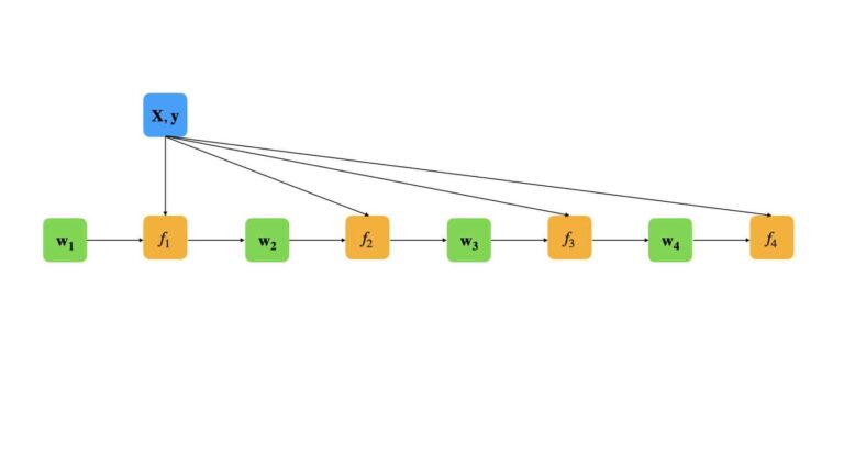
In this fashion, the errors in each successive weak learner are accounted for in the associated weights vector $\bold{w}$ . As a result, each successive model in the ensemble focuses more on the misclassified cases from earlier in the sequence.

This leaves an open question: how are we to update $\bold{w}$ ? Here we will introduce the learning rate $\alpha$ . This hyperparameter will be used here to determine the magnitude of the update to $\bold{w}$ at each point in the ensemble sequence. Normally, values of $\alpha$ range from 0.1 to 0.0001. The key here is to learn slowly, so as to avoid overfitting. The learning rate needs to be balanced with the other important hyperparameter here: the number of elements in the ensemble $n$ . Typically, $\alpha$ and $n$ need to be balanced off one another to obtain the best results.

We can now put this all together to yield a simple boosting algorithm for classification:

Initialise the ensemble $E(\bold{x}) = 0$ and the sample weights $\bold{w} = 1/M$ , where $M$ is the number of samples in the training data
Iterate through the i = 1…n models in the ensemble:
- Fit the weak learner $f_i$ to { $\bold{X},\bold{y}$ } using the sample weights $\bold{w}$
- Produce output $\hat{\bold{y}}$ from $f_i$ . Update the sample weights using the learning rate: $\bold{w}_{\bold{\hat{y}}\ne\bold{y}} = \bold{w}_{\bold{\hat{y}}\ne\bold{y}}e^{\alpha}$ , where $e$ is Euler’s number. Notice only the sample weights for misclassified cases are updated
- Measure the classification rate for $f_i$ with $C_i=\frac{M_{\bold{\hat{y}}=\bold{y}}}{M}$ , where $M_{\bold{\hat{y}}=\bold{y}}$ is the count of correctly classified samples
Normalise the classification rates $\hat{c_i} = \frac{C_i}{\sum_{i=1}^{n}C_i}$
Produce the trained boosted model: $E(\bold{x}) = \sum_{i=1}^{n}\hat{c_i}f_i(\bold{x})$

Implementation of Simple Boosting Classification in Python

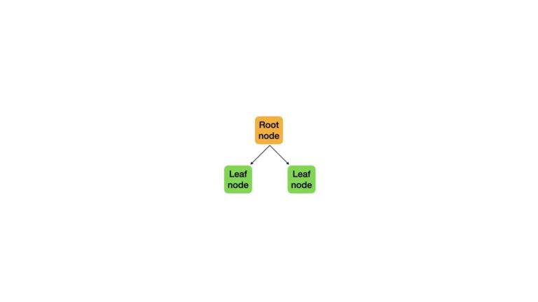
Now let’s put what we’ve learned in the previous section to practice! First, it’s important to note that our boosting algorithm does not specify the form of $f_i$ . The only thing we know is that it is a weak learner. In practice, $f_i$ is almost always a decision tree with a limited number of splits. It is common to use trees with just 1 split: a decision stump:

Let’s begin by importing all the required packages:

## imports ##
import numpy as np
import pandas as pd
from typing import Dict, Any, List
from sklearn.base import clone
import matplotlib.pyplot as plt
from sklearn.datasets import load_breast_cancer
from sklearn.model_selection import StratifiedKFold,cross_validate
from sklearn.tree import DecisionTreeClassifier
from sklearn.metrics import accuracy_score,precision_score,recall_score,f1_score,make_scorer
from sklearn.ensemble import RandomForestClassifier

Model Implementation

I will encapsulate the algorithm outlined earlier in a single class, BoostingClassifier. Let’s now look into the details of the implementation:

## boosting classifier ##
class BoostingClassifier(object):
    #initializer
    def __init__(self, 
                 weak_learner : Any, 
                 n_elements : int = 100, 
                 learning_rate : float = 0.01, 
                 record_training_f1 : bool = False) -> None:
        self.weak_learner  = weak_learner
        self.n_elements    = n_elements
        self.learning_rate = learning_rate
        self.f             = []
        self.model_weights = []
        self.f1s           = []
        self.record_f1s    = record_training_f1
        
    #destructor
    def __del__(self) -> None:
        del self.weak_learner
        del self.n_elements
        del self.learning_rate
        del self.f
        del self.model_weights
        del self.f1s

Here we see the class defined, along with its initialiser and destructor functions:

__init__(self,weak_learner,n_elements,learning_rate,record_training_f1) : this private function initialises the class instance and takes in as arguments the weak learner model (weak_learner), and the hyperparameters specifying the number of elements (n_elements) in the ensemble as well as the learning rate (learning_rate). The boolean record_training_f1 is used to control if the F1 scores will be stored while growing the ensemble during training.
__del__(self) : this private function cleans up resources allocated to the class instance when the object is deleted.

    #public function to return model parameters
    def get_params(self, deep : bool = False) -> Dict:
        return {'weak_learner':self.weak_learner,'n_elements':self.n_elements,'learning_rate':self.learning_rate}
    
    #public function to train the ensemble
    def fit(self, X_train : np.array, y_train : np.array) -> None:
        #initialize sample weights, residuals, & model array
        w              = np.ones((y_train.shape[0]))
        self.residuals = []
        self.f         = []
        #loop through the specified number of iterations in the ensemble
        for _ in range(self.n_elements):
            #make a copy of the weak learner
            model = clone(self.weak_learner)
            #fit the weak learner on the current dataset
            model.fit(X_train,y_train,sample_weight=w)
            #update the sample weights
            y_pred = model.predict(X_train)
            m      = y_pred != y_train
            w[m]  *= np.exp(self.learning_rate)
            #append resulting model
            self.f.append(model)
            #append current count of correctly labeled samples
            self.model_weights.append(np.sum(y_pred == y_train))
            #append current f1 score
            if self.record_f1s:
                self.f1s.append(self.__compute_f1(X_train,y_train))
        #normalize the model weights
        self.model_weights /= np.sum(self.model_weights)

get_params(self,deep) : this is a public function to return the input arguments when an object instance is created (this is necessary for using BoostingClassifier instances in scikit-learn functions).
fit(self,X_train,y_train) : this is a public function used to train the ensemble on the set of training predictors (X_train) and associated labels (y_train). The code here carries out the logic defined in the 4-step process at the end of the previous section.

    # private function to compute f1 score for n-trained weak learners
    def __compute_f1(self, X_train : np.array, y_train : np.array) -> float:
        #initialize output
        y_pred = np.zeros((X_train.shape[0]))
        #normalize model weights
        n_model_weights = self.model_weights/np.sum(self.model_weights)
        #traverse ensemble to generate predictions
        for model,mw in zip(self.f,n_model_weights):
            y_pred += mw*model.predict_proba(X_train)[:,1]
        #combine output from ensemble
        y_pred = np.round(y_pred).astype(int)
        #return computed f1 score
        return(f1_score(y_train,y_pred))
    
    #public function to return training f1 scores
    def get_f1s(self) -> List:
        return(self.f1s)
    
    #public function to generate predictions
    def predict(self, X_test : np.array) -> np.array:
        #initialize output
        y_pred = np.zeros((X_test.shape[0]))
        #traverse ensemble to generate predictions
        for model,mw in zip(self.f,self.model_weights):
            y_pred += mw*model.predict_proba(X_test)[:,1]
        #combine output from ensemble
        y_pred = np.round(y_pred).astype(int)
        #return predictions
        return(y_pred)

__compute_f1(self,X_train,y_train) : this private function is used to compute the F1 score for the ensemble at a specific moment during training.
get_f1s(self): this is a public function used to retrieve F1 scores calculated during training.
predict(self,X_test) : a public function to produce predictions from the trained ensemble model, using the set of predictors X_test.

Model Analysis

Now that we have an implementation of our algorithm, let’s test it out. To achieve this, I will use the Wisconsin Breast Cancer dataset. As I have already investigated these data in the article on Logistic Regression, I will not repeat that work here.

To start, let’s load in these data:

## load classification dataset
data = load_breast_cancer()
X    = data.data
y    = data.target

We can also specify the weak learner to be used here, which will be a classification decision stump:

## initialize a weak learner ##
weak_m = DecisionTreeClassifier(max_depth=1)

And finally, we can define the set of learning rates that we will use:

## set the learning rates to try ##
learning_rates = [0.1,0.01,0.001,0.0001]

Investigate Model Performance During Training

I now want to check how the model performs as more weak learners are added to the ensemble. To this end, we will record the F1 score on the training data as each weak learner is added. For this investigation, I will fix the number of weak learners to $n=100$ :

## loop through the learning rates, record F1 scores ##
dfF1 = pd.DataFrame()
for lr in learning_rates:

    #declare a boosting regressor
    clf = BoostingClassifier(weak_learner=weak_m, n_elements=100, learning_rate=lr, record_training_f1=True)
    
    #fit the model
    clf.fit(X,y)
    
    #record F1 scores
    dfF1[str(lr)] = clf.get_f1s()

The F1 scores for each learning rate are stored in the pandas dataframe dfF1. We can now easily visualise the results:

## plot the F1 scores ##
dfF1.plot()
plt.title('F1 score by Number of Component Trees in Boosting Ensemble')
plt.xlabel('Number of Component Trees')
plt.ylabel('F1 Score')
plt.show()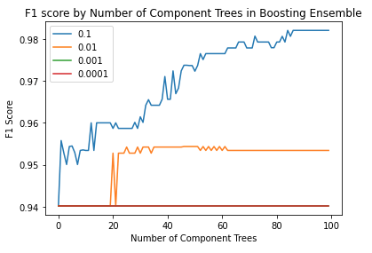

We can see that the F1 scores tend to increase with the addition of more weak learners. However, this increase is only apparent in the larger learning rates ( $\alpha = 0.1$ and $\alpha = 0.01$ ). Let’s rerun the above code, but increase the number of elements in the ensemble to $n=1000$ :

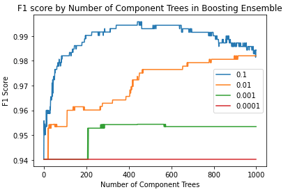
This plot is quite a lot more interesting than the first. First, we can see an increase in the F1 score for learning rate $\alpha=0.001$ , around the $n=200$ point. For the largest learning rate, we see an optimum around $n=400$ . Afterwards, the F1 score decreases; thereby showing signs of overfitting. It is clear that the smallest learning rate attempted here ( $\alpha=0.0001$ ) is not suitable for the present analysis.

Investigate Performance

Here we will use 10-fold cross validation to measure the performance of our boosting classifier. We will repeat this analysis for each of the 4 learning rates defined earlier. Let’s set the number of weak learners in the ensemble to 100:

## define the scoring metrics ##
scoring_metrics = {'accuracy' : make_scorer(accuracy_score), 
                   'precision': make_scorer(precision_score),
                   'recall'   : make_scorer(recall_score),
                   'f1'       : make_scorer(f1_score)}

## loop through each learning rate & evaluate for n_elements=100 ##
for lr in learning_rates:
    #define the model
    clf = BoostingClassifier(weak_learner=weak_m, n_elements=100, learning_rate=lr)
    #cross validate
    dcScores = cross_validate(clf,X,y,cv=StratifiedKFold(10),scoring=scoring_metrics)
    #report results
    print('Learning Rate: ',lr)
    print('Mean Accuracy: %.2f' % np.mean(dcScores['test_accuracy']))
    print('Mean Precision: %.2f' % np.mean(dcScores['test_precision']))
    print('Mean Recall: %.2f' % np.mean(dcScores['test_recall']))
    print('Mean F1: %.2f' % np.mean(dcScores['test_f1']))
    print('')

Learning Rate: 0.1

Mean Accuracy: 0.96

Mean Precision: 0.96

Mean Recall: 0.98

Mean F1: 0.97

Learning Rate: 0.01

Mean Accuracy: 0.92

Mean Precision: 0.92

Mean Recall: 0.96

Mean F1: 0.94

Learning Rate: 0.001

Mean Accuracy: 0.89

Mean Precision: 0.90

Mean Recall: 0.95

Mean F1: 0.92

Learning Rate: 0.0001

Mean Accuracy: 0.89

Mean Precision: 0.90

Mean Recall: 0.95

Mean F1: 0.92

I also re-ran the above code for an ensemble of 1000. The results of both runs are summarised below:

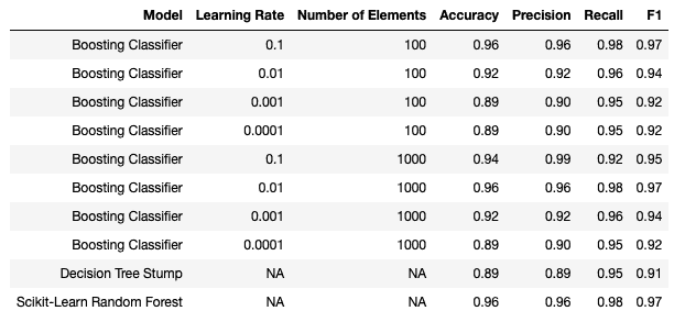
Note that the performance of a lone regression decision stump, as well as a Random Forest, are included.

Best performance is seen with two configurations of our boosting classifier: $\alpha=0.1, n=100$ and $\alpha=0.01, n=1000$ . This simple boosting model performed to similarly as the scikit-learn random forest on these data. As a point of comparison, note that the lone decision tree stump was significantly less effective. This illustrates the power of boosting.

Something curious happens when the number of elements is increased to $n=1000$ . The model with $\alpha=0.1$ shows a decrease in performance with respect to its $n=100$ counterpart. Instead, a smaller learning rate ( $\alpha=0.01$ ) now shows optimal results. What has happened is that the ( $n=1000$ , $\alpha=0.1$ ) model has overfit the data. The increased number of weak learners, in the ensemble, requires a smaller learning rate to optimally fit the data ( $\alpha=0.01$ ). Even smaller learning rates ( $\alpha<0.01$ ) also show poor performance, due to underfitting. Generally speaking, the learning rate $\alpha$ and number of weak learners $n$ , need to be balanced to achieve good results.

Final Remarks

In this post we covered an introduction to simple boosting classification in Python. The key components to this article includes:

The motivation and background for boosting ensembles
The algorithm for a basic boosting classification ensemble
How to implement the algorithm for simple boosting classification in Python
The importance of the learning rate ( $\alpha$ ) – number of weak learner ( $n$ ) trade-off

I sincerely hope you enjoyed this article, and learned something from it. Please check out my GitHub page for the code presented here, and in my other articles.

Cookie	Duration	Description
cookielawinfo-checkbox-analytics	11 months	This cookie is set by GDPR Cookie Consent plugin. The cookie is used to store the user consent for the cookies in the category "Analytics".
cookielawinfo-checkbox-functional	11 months	The cookie is set by GDPR cookie consent to record the user consent for the cookies in the category "Functional".
cookielawinfo-checkbox-necessary	11 months	This cookie is set by GDPR Cookie Consent plugin. The cookies is used to store the user consent for the cookies in the category "Necessary".
cookielawinfo-checkbox-others	11 months	This cookie is set by GDPR Cookie Consent plugin. The cookie is used to store the user consent for the cookies in the category "Other.
cookielawinfo-checkbox-performance	11 months	This cookie is set by GDPR Cookie Consent plugin. The cookie is used to store the user consent for the cookies in the category "Performance".
viewed_cookie_policy	11 months	The cookie is set by the GDPR Cookie Consent plugin and is used to store whether or not user has consented to the use of cookies. It does not store any personal data.