Implement the KNN Algorithm in Python from Scratch

In this post, we will cover the K Nearest Neighbours algorithm: how it works and how it can be used. We will work through implementing this algorithm in Python from scratch, and verify that our model works as expected.

Table of Contents

What is the KNN Algorithm?

K Nearest Neighbours (KNN) is a supervised machine learning algorithm that makes predictions based on the $K$ ‘closest‘ training data points to our point of interest, in data space. We evaluate the closest data points through the use of a distance metric, of which there are a variety of options. This algorithm is perhaps one of the simplest in machine learning, and can be used for both classification and regression problems. KNN was initially developed by Evelyn Fix & Joseph Hodges in 1951.

Being a relatively simple non-parametric algorithm, KNN’s strength is its explainability to a non-technical audience, and computational speed. However these advantages typically come at the expense of performance, when compared to more sophisticated learning algorithms.

Assumptions and Considerations

When implementing the KNN algorithm in Python from scratch, we will have to keep in mind the following points:

KNN depends on distance measures. As such, the matrix of predictor features $\bold{X}$ should be normalised prior to training the model. This is to prevent erroneous results due to large differences in scale among the input features.
The model can be sensitive to local structure in the data.
Weights can be assigned to each neighbour to enhance performance. One popular option is to use the inverse of the distance $1/d$ . Using such a weighting scheme can assist when dealing with skewed data. Another option is to assign unitary weights to each neighbour.
The presence of noisy/irrelevant features can also adversely affect performance.
KNN is prone to high variance and low bias. The choice of $K$ can address this to a certain degree. A large value reduces noise in the model output, but this also makes the distinction between different regions in the data space less clear.

Derivation of the KNN Algorithm

We can best start this discussion through illustrations. Imagine a dataset consisting of a distribution of red and black dots. Our task is to use KNN to predict what kind of dot is expected at the location of the blue circle:

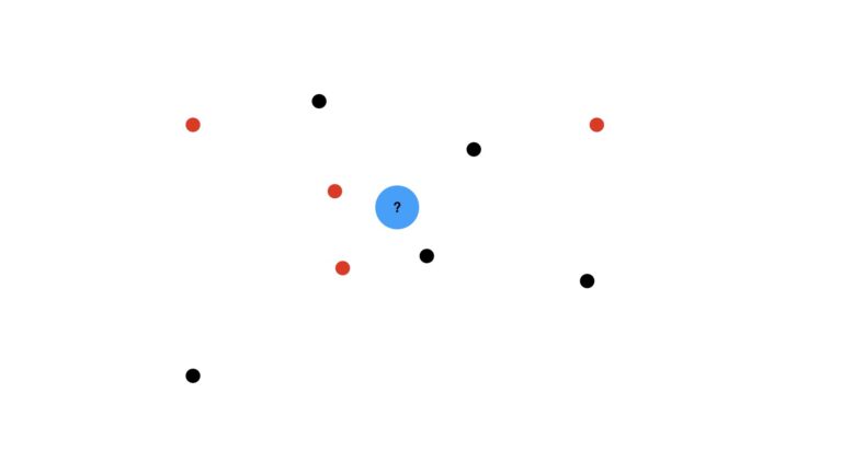
We’ll use the majority vote (mode) of the nearest data points to make this prediction. I will also assume that we’re using unitary weights per data point (i.e. each data point has equal weight in our analysis). First let’s visualise the case where we use the three closest neighbours, $K = 3$ :

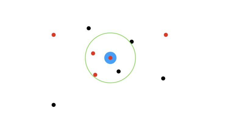
Here the green circle indicates the zone encompassing the three closest dots to the target blue circle. As the three encircled points consist of two red dots and one black, our prediction then is for a red dot.

How would our prediction change if we set $K = 5$ ?

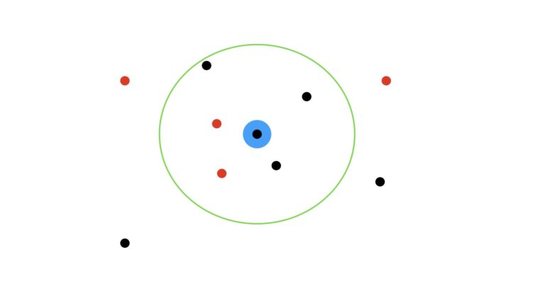
Now in this scenario, we have three black dots within the green circle, and two red dots. As such, the prediction now switches to a black dot.

The above examples illustrate the operation of KNN for classification problems. You might ask yourself, “what happens if $K$ is an even number, and we have an equal amount of red and black dots”? In this case, one of the possibilities will be selected, depending on the specifics of how the mode calculation is implemented.

The algorithm works similarly for regression, except that the mode is typically replaced by the mean. In general, both for classification and regression problems, prediction calculations are done by weighting each of the samples in some fashion.

To determine what the nearest neighbours are, a distance metric is needed. Two popular options are the Minkowski distance and Cosine distance. The Minkowski distance is actually a family of metrics that are defined by:

$d = \sqrt{\sum_i^N|a_i – b_i|^p}^{1/p}$ (1)

where $\bold{A} = (a_1, a_2, … a_N)$ and $\bold{B} = (b_1, b_2, … b_N)$ are two points in a $N$ dimensional data space. The parameter $p$ controls the specific form of the distance calculation, and is normally $p \ge 1$ . For $p = 1$ , we have the Manhattan distance. For $p = 2$ , we have the Euclidean distance.

The Cosine distance is defined as:

$d = 1 – \textrm{cosine} \: \textrm{similarity}$

$d = 1 – \frac{\sum_i^N{a_i b_i}}{ \sqrt{\sum_i^N a^2_i} \sqrt{\sum_i^N b^2_i}}$ (2)

Let’s now define our training and prediction procedures. The training procedure is quite simple:

Store the input training data $(\bold{X},\bold{y})$ , where $\bold{X}$ is the matrix of predictors and $\bold{y}$ is the vector of labels.

To generate predictions for a set of predictors $\bold{X}'$ , we can work through the following:

For each sample $\bold{x} \in \bold{X}'$ :

Compute the distance $d$ to every point in the training data $\bold{X}$ .
Extract the labels from $\bold{y}$ that correspond to the smallest $K$ distances.
For regression, compute the mean of the selected labels. For classification, compute the mode of the selected labels.

Implementation of a KNN Classifier & Regressor

With our methodology defined in the previous section, we can now proceed to implement the KNN algorithm in Python from scratch. This implementation will cover both regression and classification use cases. Let’s start by importing the packages needed for our KNN model:

import numpy as np
from scipy import stats
from typing import Dict, Any
from abc import ABC,abstractmethod

I will now define a base class, that will cover all the functionality common to regression and classification use cases:

class KNN(ABC):
    """
    Base class for KNN implementations
    """
    
    def __init__(self, K : int = 3, metric : str = 'minkowski', p : int = 2) -> None:
        """
        Initializer function. Ensure that input parameters are compatiable.
        Inputs:
            K      -> integer specifying number of neighbours to consider
            metric -> string to indicate the distance metric to use (valid entries are 'minkowski' or 'cosine')
            p      -> order of the minkowski metric (valid only when distance == 'minkowski')
        """
        # check distance is a valid entry
        valid_distance = ['minkowski','cosine']
        if metric not in valid_distance:
            msg = "Entered value for metric is not valid. Pick one of {}".format(valid_distance)
            raise ValueError(msg)
        # check minkowski p parameter
        if (metric == 'minkowski') and (p <= 0):
            msg = "Entered value for p is not valid. For metric = 'minkowski', p >= 1"
            raise ValueError(msg)
        # store/initialise input parameters
        self.K       = K
        self.metric  = metric
        self.p       = p
        self.X_train = np.array([])
        self.y_train = np.array([])
        
    def __del__(self) -> None:
        """
        Destructor function. 
        """
        del self.K
        del self.metric
        del self.p
        del self.X_train
        del self.y_train
      
    def __minkowski(self, x : np.array) -> np.array:
        """
        Private function to compute the minkowski distance between point x and the training data X
        Inputs:
            x -> numpy data point of predictors to consider
        Outputs:
            np.array -> numpy array of the computed distances
        """
        return np.power(np.sum(np.power(np.abs(self.X_train - x),self.p),axis=1),1/self.p)
    
    def __cosine(self, x : np.array) -> np.array:
        """
        Private function to compute the cosine distance between point x and the training data X
        Inputs:
            x -> numpy data point of predictors to consider
        Outputs:
            np.array -> numpy array of the computed distances
        """
        return (1 - (np.dot(self.X_train,x)/(np.linalg.norm(x)*np.linalg.norm(self.X_train,axis=1))))
    
    def __distances(self, X : np.array) -> np.array:
        """
        Private function to compute distances to each point x in X[x,:]
        Inputs:
            X -> numpy array of points [x]
        Outputs:
            D -> numpy array containing distances from x to all points in the training set.
        """
        # cover distance calculation
        if self.metric == 'minkowski':
            D = np.apply_along_axis(self.__minkowski,1,X)
        elif self.metric == 'cosine':
            D = np.apply_along_axis(self.__cosine,1,X)
        # return computed distances
        return D
    
    @abstractmethod
    def _generate_predictions(self, idx_neighbours : np.array) -> np.array:
        """
        Protected function to compute predictions from the K nearest neighbours
        """
        pass
        
    def fit(self, X : np.array, y : np.array) -> None:
        """
        Public training function for the class. It is assummed input X has been normalised.
        Inputs:
            X -> numpy array containing the predictor features
            y -> numpy array containing the labels associated with each value in X
        """
        # store training data
        self.X_train = np.copy(X)
        self.y_train = np.copy(y)
        
    def predict(self, X : np.array) -> np.array:
        """
        Public prediction function for the class. 
        It is assummed input X has been normalised in the same fashion as the input to the training function
        Inputs:
            X -> numpy array containing the predictor features
        Outputs:
           y_pred -> numpy array containing the predicted labels
        """
        # ensure we have already trained the instance
        if (self.X_train.size == 0) or (self.y_train.size == 0):
            raise Exception('Model is not trained. Call fit before calling predict.')
        # compute distances
        D = self.__distances(X)
        # obtain indices for the K nearest neighbours
        idx_neighbours = D.argsort()[:,:self.K]
        # compute predictions
        y_pred = self._generate_predictions(idx_neighbours)
        # return results
        return y_pred
    
    def get_params(self, deep : bool = False) -> Dict:
        """
        Public function to return model parameters
        Inputs:
            deep -> boolean input parameter
        Outputs:
            Dict -> dictionary of stored class input parameters
        """
        return {'K':self.K,
                'metric':self.metric,
                'p':self.p}

__init__(self, K, metric, p) : Initialiser function that is called when a class instance is created. Input arguments include:
1. K, the integer number of nearest neighbours to consider
2. metric, the type of distance metric to use (must be either ‘minkowski’ or ‘cosine’)
3. p, integer parameter when metric = ‘minkowski’ (must be greater than or equal to 1)
__del__(self) : Destructor function used to release resources when a class instance is removed
__minkowski(self, x) : Private function used to compute (1). The input x is $\bold{x} \in \bold{X}'$ mentioned in the previous section.
__cosine(self, x) : Private function used to compute (2). The input x is $\bold{x} \in \bold{X}'$ mentioned in the previous section.
__distances(self, X) : Private function used to compute distances when generating predictions. The input X is $\bold{X}'$ mentioned in the previous section.
_generate_predictions(self, idx_neighbours) : Protected function used to generate predictions, using the $K$ nearest neighbours as indexed in idx_neighbours. This function is implemented in daughter classes.
fit(self, X, y) : Public function that executes our training procedure. Input arguments X and y correspond to $(\bold{X},\bold{y})$ from the previous section.
predict(self, X) : Public function used to execute our prediction procedure. The input matrix X is the set of predictors $\bold{X}'$ mentioned previously.
get_params(self, deep) : Public function used to return the instance input parameters. This is required for use with scikit-learn functionality.

Let’s now define a daughter class, for the classification use case:

class KNNClassifier(KNN):
    """
    Class for KNN classifiction implementation
    """
    
    def __init__(self, K : int = 3, metric : str = 'minkowski', p : int = 2) -> None:
        """
        Initializer function. Ensure that input parameters are compatiable.
        Inputs:
            K       -> integer specifying number of neighbours to consider
            metric  -> string to indicate the distance metric to use (valid entries are 'minkowski' or 'cosine')
            p       -> order of the minkowski metric (valid only when distance == 'minkowski')
        """
        # call base class initialiser
        super().__init__(K,metric,p)
        
    def _generate_predictions(self, idx_neighbours : np.array) -> np.array:
        """
        Protected function to compute predictions from the K nearest neighbours
        Inputs:
            idx_neighbours -> indices of nearest neighbours
        Outputs:
            y_pred -> numpy array of prediction results
        """        
        # compute the mode label for each submitted sample
        y_pred = stats.mode(self.y_train[idx_neighbours],axis=1).mode.flatten()   
        # return result
        return y_pred

__init__(self, K, metric, p) : Initialiser function, which calls the base class initialiser.
_generate_predictions(self, idx_neighbours) : Protected function used to generate predictions, using the $K$ nearest neighbours as indexed in idx_neighbours. The mode of the selected labels is calculated here, and returned. Note that each selected label has equal weight in this calculation.

Finally, we can proceed to the regressor daughter class implementation:

class KNNRegressor(KNN):
    """
    Class for KNN regression implementation
    """
    
    def __init__(self, K : int = 3, metric : str = 'minkowski', p : int = 2) -> None:
        """
        Initializer function. Ensure that input parameters are compatiable.
        Inputs:
            K       -> integer specifying number of neighbours to consider
            metric  -> string to indicate the distance metric to use (valid entries are 'minkowski' and 'cosine')
            p       -> order of the minkowski metric (valid only when distance == 'minkowski')
        """
        # call base class initialiser
        super().__init__(K,metric,p)
        
    def _generate_predictions(self, idx_neighbours : np.array) -> np.array:
        """
        Protected function to compute predictions from the K nearest neighbours
        Inputs:
            idx_neighbours -> indices of nearest neighbours
        Outputs:
            y_pred -> numpy array of prediction results
        """
        # compute the mean label for each submitted sample
        y_pred = np.mean(self.y_train[idx_neighbours],axis=1)         
        # return result
        return y_pred

__init__(self, K, metric, p) : Initialiser function, which calls the base class initialiser.
_generate_predictions(self, idx_neighbours) : Protected function used to generate predictions, using the $K$ nearest neighbours as indexed in idx_neighbours. The mean of the selected labels is calculated here, and returned. Note that each selected label has equal weight in this calculation.

Testing Performance

With our KNN algorithm implemented, let’s now proceed to check how it performs on some data. I will start with the classification problem.

Testing the KNN Classifier

We can begin by importing some data. Here I’ll load the breast cancer dataset. A full description of these data can be found here. Note I already analysed these data in my previous article on Logistic Regression. As such, I won’t repeat that work here.

## load classification dataset ##
data = load_breast_cancer()
X    = data.data
y    = data.target

# properly format labels
y = np.where(y==0,-1,1)

I will use 10-fold cross-validation to measure the performance of the KNN classifier. We will also try a variety of values for $K$ , and the distance measures. A custom scorer and helper function can assist us here:

## define the scoring metrics ##
scoring_metrics = {'accuracy' : make_scorer(accuracy_score), 
                   'precision': make_scorer(precision_score),
                   'recall'   : make_scorer(recall_score),
                   'f1'       : make_scorer(f1_score)}
                   
## define a helper function for our analysis ##
def cv_classifier_analysis(pipe : Any, 
                           X : np.array, 
                           y : np.array, 
                           k : int, 
                           scoring_metrics : Dict,
                           metric : str) -> None:
    """
    Function to carry out cross-validation analysis for input KNN classifier
    Inputs:
        pipe            -> input pipeline containing preprocessing and KNN classifier
        X               -> numpy array of predictors
        y               -> numpy array of labels
        k               -> integer value for number of nearest neighbours to consider
        scoring_metrics -> dictionary of scoring metrics to consider 
        metric          -> string indicating distance metric used
    """
    # print hyperparameter configuration
    print('RESULTS FOR K = {0}, {1}'.format(k,metric))
    # run cross validation
    dcScores = cross_validate(pipe,X,y,cv=StratifiedKFold(10),scoring=scoring_metrics)
    # report results
    print('Mean Accuracy: %.2f' % np.mean(dcScores['test_accuracy']))
    print('Mean Precision: %.2f' % np.mean(dcScores['test_precision']))
    print('Mean Recall: %.2f' % np.mean(dcScores['test_recall']))
    print('Mean F1: %.2f' % np.mean(dcScores['test_f1']))

The custom scorer will measure the accuracy, precision, recall, and F1 score during our analysis. Note that the helper function expects a Pipeline as input. This pipeline will consist of a Standard Scaler, to normalise the input features, followed by the KNN model. Let’s now write the portion of code that will carry out the test for our custom implementation:

## perform cross-validation for a range of model hyperparameters for the Custom model ##
K = [3,6,9]
for k in K:
    # define the pipeline for manhatten distance
    p_manhat = Pipeline([('scaler', StandardScaler()), ('knn', KNNClassifier(k, metric = 'minkowski', p = 1))])
    # define the pipeline for euclidean distance
    p_euclid = Pipeline([('scaler', StandardScaler()), ('knn', KNNClassifier(k, metric = 'minkowski', p = 2))])
    # define the pipeline for cosine distance
    p_cosine = Pipeline([('scaler', StandardScaler()), ('knn', KNNClassifier(k, metric = 'cosine'))])
    # cross validate for p_manhat
    cv_classifier_analysis(p_manhat, X, y, k, scoring_metrics, 'MANHATTEN DISTANCE')
    # cross validate for p_euclid
    cv_classifier_analysis(p_euclid, X, y, k, scoring_metrics, 'EUCLIDEAN DISTANCE')
    # cross validate for p_cosine
    cv_classifier_analysis(p_cosine, X, y, k, scoring_metrics, 'COSINE DISTANCE')

We can also write a similar piece of code for the scikit-learn KNN classifier, to compare with our custom model:

## perform cross-validation for a range of model hyperparameters for the Scikit-learn model ##
K = [3,6,9]
for k in K:
    # define the model for manhatten distance
    p_manhat = Pipeline([('scaler', StandardScaler()), ('knn', KNeighborsClassifier(k, metric = 'minkowski', p = 1))])
    # define the model for euclidean distance
    p_euclid = Pipeline([('scaler', StandardScaler()), ('knn', KNeighborsClassifier(k, metric = 'minkowski', p = 2))])
    # define the model for cosine distance
    p_cosine = Pipeline([('scaler', StandardScaler()), ('knn', KNeighborsClassifier(k, metric = 'cosine'))])
    # cross validate for m_manhat
    cv_classifier_analysis(p_manhat, X, y, k, scoring_metrics, 'MANHATTEN DISTANCE')
    # cross validate for m_euclid
    cv_classifier_analysis(p_euclid, X, y, k, scoring_metrics, 'EUCLIDEAN DISTANCE')
    # cross validate for m_cosine
    cv_classifier_analysis(p_cosine, X, y, k, scoring_metrics, 'COSINE DISTANCE')

Running both of the previous sections of code yields the following tabulated results:

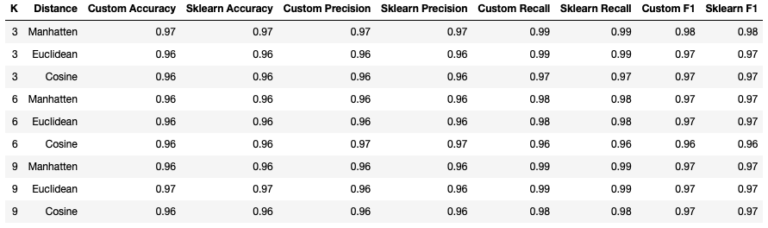
Firstly, it’s clear that our custom KNN classifier yields results that are identicial to the scikit-learn implementation. Looking at the statistics tabulated, it appears that using the Manhatten distance with $K = 3$ produces the best results. However, it should be clear that the performance of the KNN classifiers appears to vary little, with the choice of hyperparameters analysed here.

Testing the KNN Regressor

The analysis in this subsection will be similar to the previous, but here I will load in the diabetes dataset. A full description of this dataset is available here. Note I have already explored these data in my previous article on Adaboost Regression. As such, I won’t repeat that analysis here.

## load regression dataset ##
X,y = load_diabetes(return_X_y=True,as_frame=False)

Like before, I will use 10-fold cross-validation to measure the performance of the KNN regressor for a variety of hyper parameter values. A custom scorer and helper function, similar to those used for the classifier, will also assist us here:

## define the scoring metrics ##
scoring_metrics = {'mse' : make_scorer(mean_squared_error), 
                   'mae': make_scorer(mean_absolute_error)}
                   
## define a helper function for our analysis ##
def cv_regressor_analysis(pipe : Any, 
                          X : np.array, 
                          y : np.array, 
                          k : int, 
                          scoring_metrics : Dict,
                          metric : str) -> None:
    """
    Function to carry out cross-validation analysis for input KNN regressor
    Inputs:
        pipe            -> input pipeline containing preprocessing and KNN regressor
        X               -> numpy array of predictors
        y               -> numpy array of labels
        k               -> integer value for number of nearest neighbours to consider
        scoring_metrics -> dictionary of scoring metrics to consider 
        metric          -> string indicating distance metric used
    """
    # print hyperparameter configuration
    print('RESULTS FOR K = {0}, {1}'.format(k,metric))
    # run cross validation
    dcScores = cross_validate(pipe,X,y,cv=10,scoring=scoring_metrics)
    # report results
    print('Mean MSE: %.2f' % np.mean(dcScores['test_mse']))
    print('Mean MAE: %.2f' % np.mean(dcScores['test_mae']))

The custom scorer will measure the mean squared error (MSE) and mean absolute error (MAE) during our analysis. Let’s now write the portion of code that will carry out the test for our custom implementation:

## perform cross-validation for a range of model hyperparameters for the Custom model ##
K = [3,6,9]
for k in K:       
    # define the pipeline for manhatten distance
    p_manhat = Pipeline([('scaler', StandardScaler()), ('knn', KNNRegressor(k, metric = 'minkowski', p = 1))])
    # define the pipeline for euclidean distance
    p_euclid = Pipeline([('scaler', StandardScaler()), ('knn', KNNRegressor(k, metric = 'minkowski', p = 2))])
    # define the pipeline for cosine distance
    p_cosine = Pipeline([('scaler', StandardScaler()), ('knn', KNNRegressor(k, metric = 'cosine'))])
    # cross validate for p_manhat
    cv_regressor_analysis(p_manhat, X, y, k, scoring_metrics, 'MANHATTEN DISTANCE')
    # cross validate for p_euclid
    cv_regressor_analysis(p_euclid, X, y, k, scoring_metrics, 'EUCLIDEAN DISTANCE')
    # cross validate for p_cosine
    cv_regressor_analysis(p_cosine, X, y, k, scoring_metrics, 'COSINE DISTANCE')

We can also write a similar piece of code for the scikit-learn KNN regressor, to compare with our custom model:

## perform cross-validation for a range of model hyperparameters for the Scikit-learn model ##
K = [3,6,9]    
for k in K:       
    # define the pipeline for manhatten distance
    p_manhat = Pipeline([('scaler', StandardScaler()), ('knn', KNeighborsRegressor(k, metric = 'minkowski', p = 1))])
    # define the pipeline for euclidean distance
    p_euclid = Pipeline([('scaler', StandardScaler()), ('knn', KNeighborsRegressor(k, metric = 'minkowski', p = 2))])
    # define the pipeline for cosine distance
    p_cosine = Pipeline([('scaler', StandardScaler()), ('knn', KNeighborsRegressor(k, metric = 'cosine'))])
    # cross validate for p_manhat
    cv_regressor_analysis(p_manhat, X, y, k, scoring_metrics, 'MANHATTEN DISTANCE')
    # cross validate for p_euclid
    cv_regressor_analysis(p_euclid, X, y, k, scoring_metrics, 'EUCLIDEAN DISTANCE')
    # cross validate for p_cosine
    cv_regressor_analysis(p_cosine, X, y, k, scoring_metrics, 'COSINE DISTANCE')

Running both of the previous sections of code yields the following tabulated results:

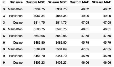
Like the situation with the KNN classifier, it is clear that our custom KNN regressor yields results that are identicial to the scikit-learn implementation. Looking at the statistics tabulated, it appears that performance improves as $K$ increases across all distance settings, with optimal values being seen for $K = 9$ $K = 9$ . Of the distance metrics attempted, the Cosine distance yields the best results for both MSE and MAE. At the same time, the Euclidean distance with $K = 3$ $K = 9$ produces the worst set of results for these data.

Final Remarks

In this article you have learned:

What is the K Nearest Neighbours algorithm, and when it was developed
The assumptions and considerations that need to be kept in mind when using this algorithm
A derivation of KNN
How to implement the KNN algorithm in Python from scratch
How our implementation of KNN compares against the models available from scikit-learn

I hope you enjoyed this article, and gained some value from it. If you would like to take a closer look at the code presented here, please take a look at my GitHub. If you have any questions or suggestions, please feel free to add a comment below. Your input is greatly appreciated.

Hi I'm Michael Attard, a Data Scientist with a background in Astrophysics. I enjoy helping others on their journey to learn more about machine learning, and how it can be applied in industry.

Cookie	Duration	Description
cookielawinfo-checkbox-analytics	11 months	This cookie is set by GDPR Cookie Consent plugin. The cookie is used to store the user consent for the cookies in the category "Analytics".
cookielawinfo-checkbox-functional	11 months	The cookie is set by GDPR cookie consent to record the user consent for the cookies in the category "Functional".
cookielawinfo-checkbox-necessary	11 months	This cookie is set by GDPR Cookie Consent plugin. The cookies is used to store the user consent for the cookies in the category "Necessary".
cookielawinfo-checkbox-others	11 months	This cookie is set by GDPR Cookie Consent plugin. The cookie is used to store the user consent for the cookies in the category "Other.
cookielawinfo-checkbox-performance	11 months	This cookie is set by GDPR Cookie Consent plugin. The cookie is used to store the user consent for the cookies in the category "Performance".
viewed_cookie_policy	11 months	The cookie is set by the GDPR Cookie Consent plugin and is used to store whether or not user has consented to the use of cookies. It does not store any personal data.