Unbalanced data is a common occurrence for classification problems, with significant implications for model performance. In this post, we’ll compare 4 different techniques for treating unbalanced data. All coding examples shown here are done in Python, and available on my Github.
Table of Contents

4 Techniques to Handle Unbalanced Data – image by author
Why Treat for Unbalanced Data?
Unbalanced data can represent a significant obstacle to building an effective classification model, as the training procedure will tend to favor the majority classes over the minority classes. This is due to the way learning procedures operate, where learning is typically measured against a loss function that does not take into account different frequencies for the classes involved. Unbalanced data is commonly encountered in industries such as finance and health care, to name two examples.
The 4 methods covered here include:
- Oversampling the minority class
- Undersampling the majority class
- Using synthetic data to augment the minority class
- Set class weights in the model itself
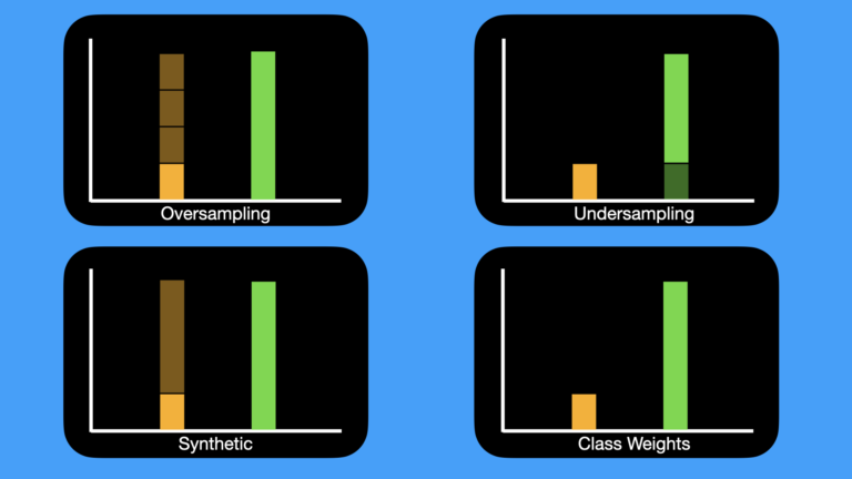
Figure 1: 4 different techniques for handling unbalanced data. Orange indicates the minority class, whereas green is the majority class. Shaded regions represent data that is added, or selected, as part of the approach.
Oversampling involves drawing samples, with replacement, from the minority class. Samples are drawn in this way until we have the same number of data points as the majority class.
With undersampling, we draw samples from the majority class, without replacement. The number of samples drawn is equal to the amount of data present in the minority class.
Instead of taking draws from the existing data, the synthetic approach involves modeling the minority class, and then using the obtained model to generate new samples. The number of samples generated is equal to the different between the majority and minority classes.
Lastly, we can avoid manipulating the training data altogether, and instead alter the training algorithm to account for the class imbalance. We can do this by assigning different class weights that are inversely proportional to the frequency of each class.
Setup the Python Experiment
We will consider a binary classification problem for our comparison. For modeling, a Random Forest Classifier will be used. Let’s import the packages required, create our data, and initialize a model:
# import packages
from typing import Dict
import pandas as pd
import matplotlib.pyplot as plt
from sklearn.model_selection import cross_validate
from sklearn.datasets import make_classification
from sklearn.ensemble import RandomForestClassifier
from sdv.single_table import GaussianCopulaSynthesizer
from sdv.metadata import Metadata

# setup dataset
X, y = make_classification(
    n_samples = 10000,
    n_features = 100,
    n_informative = 10,
    n_redundant = 40,
    n_repeated = 40,
    n_classes = 2,
    weights = [0.95, 0.05],
    random_state = 42,
    return_X_y = True
)

# package data as a single pandas dataframe
data_df = pd.DataFrame(X, columns = [f"col{i+1}" for i in range(X.shape[1])])
data_df['label'] = y

# define our model
model = RandomForestClassifier(n_estimators=10, max_depth=5, random_state=42)
Notice that the generated data is highly imbalanced, with 95% of the data in the first class, and the remaining 5% in the other. Our Random Forest consists of 10 weak learners, with a maximum depth of 5.
Baseline
Before trying out any techniques for the unbalanced data, let’s first measure how well our model performs on the data as-is. This will serve as a good point of comparison later on:
# prepare data for evaluation
X = data_df.drop('label', axis=1)
y = data_df.label

# perform cv
baseline_results = cross_validate(model, X, y, cv = 5, scoring=('roc_auc','f1'), n_jobs=-1)

baseline_results
{'fit_time': array([0.21453214, 0.21211219, 0.21194029, 0.21146607, 0.21261692]),
'score_time': array([0.00449896, 0.00428009, 0.00419688, 0.00418806, 0.00423336]),
'test_roc_auc': array([0.88977224, 0.85300239, 0.86868751, 0.85944042, 0.8647359 ]),
'test_f1': array([0.54666667, 0.52631579, 0.55128205, 0.53947368, 0.50684932])} These results aren’t the best. Let’s see if we can improve on this.
Oversampling the Minority Class
In this scenario, we sample with replacement from the minority class, until the number of samples from both classes are equal. Let’s build a function to take care of this operation:
def oversample_minority_class(data_df: pd.DataFrame, minority_class: Dict[str, int]) -> pd.DataFrame:
    """
    Function to handle an unbalanced binary dataset via minority class oversampling

    Input:
        data_df -> pandas dataframe containing the features and labels
        minority_class -> dictionary containing the label column name (key) and minority value (value)
    Output:
        pandas dataframe with equal number of samples for each class
    """
    # split the data based on the label
    label_col = list(minority_class.keys())[0]
    minority = data_df[data_df[label_col] == minority_class[label_col]].copy()
    majority = data_df[data_df[label_col] != minority_class[label_col]].copy()

    # check our classes have been processed correctly
    if minority.shape[0] > majority.shape[0]:
        msg = f"minority class not properly indicated, has {minority.shape[0]} samples while the majority class has {majority.shape[0]}"
        raise ValueError(msg)

    # sample with replacement the minority class
    sampled_minority = minority.sample(n = majority.shape[0], replace = True, random_state = 42)

    # recombine the data and return
    return pd.concat([majority, sampled_minority], axis=0).reset_index(drop=True)

# perform oversampling
oversampled_df = oversample_minority_class(data_df, {'label': 1})

# prepare data for evaluation
X = oversampled_df.drop('label', axis=1)
y = oversampled_df.label

# perform cv
oversampled_results = cross_validate(model, X, y, cv = 5, scoring=('roc_auc','f1'), n_jobs=-1)

# examine results
oversampled_results
{'fit_time': array([0.2566731 , 0.28940797, 0.29200792, 0.25867295, 0.29049706]),
'score_time': array([0.00513101, 0.00572181, 0.00557709, 0.00518394, 0.0057478 ]),
'test_roc_auc': array([0.95195767, 0.94974512, 0.94917085, 0.94773484, 0.95410516]),
'test_f1': array([0.86788155, 0.88335664, 0.86986107, 0.86623848, 0.88222098])} These results are a good improvement over the baseline. Let’s checkout the next method.
Undersampling the Majority Class
Here we’ll undersample the majority class, such that we have the same number of samples for both classes. Like before, we will contain this logic in a function:
def undersample_majority_class(data_df: pd.DataFrame, majority_class: Dict[str, int]) -> pd.DataFrame:
    """
    Function to handle an unbalanced binary dataset via majority class undersampling

    Input:
        data_df -> pandas dataframe containing the features and labels
        majority_class -> dictionary containing the label column name (key) and majority value (value)
    Output:
        pandas dataframe with equal number of samples for each class
    """
    # split the data based on the label
    label_col = list(majority_class.keys())[0]
    minority = data_df[data_df[label_col] != majority_class[label_col]].copy()
    majority = data_df[data_df[label_col] == majority_class[label_col]].copy()

    # check our classes have been processed correctly
    if minority.shape[0] > majority.shape[0]:
        msg = f"majority class not properly indicated, has {majority.shape[0]} samples while the minority class has {minority.shape[0]}"
        raise ValueError(msg)

    # sample without replacement the majority class
    sampled_majority = majority.sample(n = minority.shape[0], replace = False, random_state = 42)

    # recombine the data and return
    return pd.concat([minority, sampled_majority], axis=0).reset_index(drop=True)

# perform undersampling
undersampled_df = undersample_majority_class(data_df, {'label': 0})

# prepare data for evaluation
X = undersampled_df.drop('label', axis=1)
y = undersampled_df.label

# perform cv
undersampled_results = cross_validate(model, X, y, cv = 5, scoring=('roc_auc','f1'), n_jobs=-1)

# examine results
undersampled_results
{'fit_time': array([0.01984072, 0.02300906, 0.01970983, 0.02220488, 0.02111673]),
'score_time': array([0.0028131 , 0.00327182, 0.00285602, 0.003021 , 0.00290012]),
'test_roc_auc': array([0.91036108, 0.89104452, 0.86457369, 0.90409446, 0.91343867]),
'test_f1': array([0.85581395, 0.82178218, 0.75621891, 0.84729064, 0.79792746])} These results are not as good as what we saw with the over sampling technique. This is not too surprising since here we are leaving out quite a lot of data from the training procedure.
Synthetic Data
With this approach, we will model the minority class in order to generate synthetic samples to augment our dataset:
def synthetic_data(data_df: pd.DataFrame, minority_class: Dict[str, int]) -> pd.DataFrame:
    """
    Function to handle an unbalanced binary dataset via sythetic data generation

    Input:
        data_df -> pandas dataframe containing the features and labels
        minority_class -> dictionary containing the label column name (key) and minority value (value)
    Output:
        pandas dataframe with equal number of samples for each class
    """
    # split the data based on the label
    label_col = list(minority_class.keys())[0]
    minority = data_df[data_df[label_col] == minority_class[label_col]].copy()
    majority = data_df[data_df[label_col] != minority_class[label_col]].copy()

    # check our classes have been processed correctly
    if minority.shape[0] > majority.shape[0]:
        msg = f"minority class not properly indicated, has {minority.shape[0]} samples while the majority class has {majority.shape[0]}"
        raise ValueError(msg)

    # generate synethic samples
    X_minority = minority.drop('label', axis=1)
    metadata = Metadata.detect_from_dataframe(X_minority)
    synthesizer = GaussianCopulaSynthesizer(metadata)
    synthesizer.fit(X_minority)
    synthetic = synthesizer.sample(num_rows=(data_df.shape[0]-2*X_minority.shape[0]))
    synthetic['label'] = 1

    # recombine the data and return
    return pd.concat([majority, minority, synthetic], axis=0).reset_index(drop=True)

synthetic_df = synthetic_data(data_df, {'label': 1})

# prepare data for evaluation
X = synthetic_df.drop('label', axis=1)
y = synthetic_df.label

# perform cv
synthetic_results = cross_validate(model, X, y, cv = 5, scoring=('roc_auc','f1'), n_jobs=-1)

synthetic_results
{'fit_time': array([0.27563596, 0.39633083, 0.39413691, 0.39300394, 0.39492869]),
'score_time': array([0.00450015, 0.00531197, 0.005265 , 0.00545311, 0.00546098]),
'test_roc_auc': array([0.94296339, 0.99998547, 0.99999441, 0.99999776, 0.99999944]),
'test_f1': array([0.83235567, 0.99762721, 0.99841605, 0.99947146, 0.99841605])} These results are the best so far. I must admit I am surprised at how well this approach has worked!
Class Weights
In this scenario, we don’t modify the data at all. Instead, we’ll change the learning algorithm itself to account for the class imbalance througth the class_weight argument:
# define our model
model = RandomForestClassifier(n_estimators=10, max_depth=5, random_state=42, class_weight="balanced")

# prepare data for evaluation
X = data_df.drop('label', axis=1)
y = data_df.label

# perform cv
class_weights_results = cross_validate(model, X, y, cv = 5, scoring=('roc_auc','f1'), n_jobs=-1)

# examine results
class_weights_results
{'fit_time': array([0.23348808, 0.17996097, 0.23339891, 0.23284411, 0.2308197 ]),
'score_time': array([0.00449204, 0.00377512, 0.00442505, 0.00432992, 0.00422621]),
'test_roc_auc': array([0.91333392, 0.86931578, 0.90122939, 0.88474134, 0.89426011]),
'test_f1': array([0.60902256, 0.55905512, 0.53174603, 0.58914729, 0.54545455])} Here we see only a marginal improvement over the baseline.
Final Remarks
We tested 4 different approaches to handelling class imbalance by evaluating a Random Forest Classifier with a 5-fold cross validation. The metrics examined include the ROC-AUC and the F1 score. We can easily compare the results through the use of box plots:
# package data for plotting
auc = [
    baseline_results['test_roc_auc'].tolist(),
    oversampled_results['test_roc_auc'].tolist(),
    undersampled_results['test_roc_auc'].tolist(),
    synthetic_results['test_roc_auc'].tolist(),
    class_weights_results['test_roc_auc'].tolist()
]
f1 = [
    baseline_results['test_f1'].tolist(),
    oversampled_results['test_f1'].tolist(),
    undersampled_results['test_f1'].tolist(),
    synthetic_results['test_f1'].tolist(),
    class_weights_results['test_f1'].tolist()
]

labels = ['baseline', 'oversampled', 'undersampled', 'synthetic', 'class_weights']
plt.boxplot(auc, tick_labels=labels)
plt.ylabel('ROC AUC score')
plt.title('Distribution of ROC AUC scores per method')
plt.show()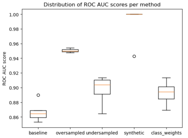
Figure 2: boxplot of ROC AUC distributions for the baseline & methods tried in this experiment
labels = ['baseline', 'oversampled', 'undersampled', 'synthetic', 'class_weights']
plt.boxplot(f1, tick_labels=labels)
plt.ylabel('F1 score')
plt.title('Distribution of F1 scores per method')
plt.show()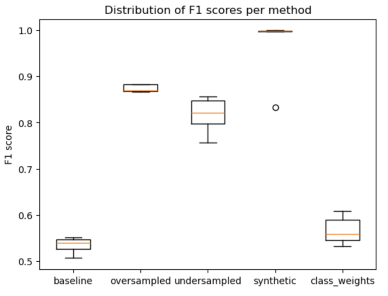
Figure 3: boxplot of the F1 scores for the baseline & methods tried in this experiment
The clear winner is the synthetic data approach, yielding excellent results with minimal spread over the 5 runs. In second place comes the oversampling approach. Going into this experiment, I was expecting the class_weights approach to do much better, as this is the single technique that does not “manipulate”, or modify, the data in any way. As it turns out, this was the worst method attempted.
I hope you enjoyed this article, and gained some value from it. If you would like to take a closer look at the code presented here, please take a look at my GitHub. If you have any questions or suggestions, please feel free to add a comment below. Your input is greatly appreciated.
Interested in signing up for my Monthly Newsletter? At the end of each month I will send out this free newsletter to each of my subscribers by email. This is the best way to stay on top of my latest content. Sign up for the newsletter here!
Related Posts
Hi I'm Michael Attard, a Data Scientist with a background in Astrophysics. I enjoy helping others on their journey to learn more about machine learning, and how it can be applied in industry.