In this article, we’ll cover an approximate method for computing Shapley Values. These are powerful quantities that help explain how machine learning models actually work. The approach we’ll take here is much more appropriate for analyzing machine learning models, as opposed to using the strict mathematical definition for Shapley Values. The method covered here is based off of the one described in Strumbelj et al. (2014). All code presented in this post can be found on my GitHub.
Table of Contents

Shapley Values for Machine Learning – image by Abi Plata
Why Use Shapley Values?
With the increasing complexity of machine learning algorithms, the need arises to be able to explain how these models arrive at their predictions. This is a critical component to any project where stakeholders/regulators demand solid, and yet understandable, explanations in order to assess a model for production. Shapley Values hold the potential to meet this demand.
In my YouTube video entitled Introduction to Shapley Values, I covered the classic definition of these quantities, originally developed within the context of Game Theory. Shapley Values provide a powerful means by which we can assess how important a given input feature is, to the output of any predictive machine learning model. As a result, Shapley Values have properties that are extremely important to developing explainable AI solutions. You can watch that video here:
The following shortcomings were discussed at the end of that video:
- As the number of input features increases, the number of computational iterations becomes exponentially larger
- Retraining our model for each value function call isn’t very sensible: many models will not function on just a subset of features, and the training times can be quite long!
Both of these points make the classic Shapley Value unusable in a practical, machine learning context. As such, what we need is to develop a numerical technique that will deliver Approximate Shapley Values, that will also circumvent the two issues raised above.
Approximate Shapley Values
The Shapley Value \phi_i, for one feature i out of all available input features, is approximately given by:
\phi_i = \frac{1}{M}\sum_{m=1}^M f(x^m_{+i}) – f(x^m_{-i}) = \frac{1}{M}\sum_{m=1}^M \phi^m_i
where:
- f is the predictive model
- M is an integer number of iterations we can pick
- x^m_{+i} is a constructed sample that includes the original value for feature i
- x^m_{-i} is a constructed sample that replaces the original value for feature i
To shed more light on this, let’s now cover the procedure to compute \phi_i, step-by-step:
- Select a value for M, i, and a sample of interest x from the available input predictive dataset X. Note X does not include labels/targets
- for m=1..M:
- A) draw a random sample z from X
- B) compute a random ordering o of the set of features in X
- C) reorder the features in samples x and z according to o, \implies x^o and z^o
- D) construct sample x^m_{+i} = (x^o_1, …, x^o_{i-1}, x^o_{i}, z^o_{i+1}, …, z^o_F)
- E) construct sample x^m_{-i} = (x^o_1, …, x^o_{i-1}, z^o_{i}, z^o_{i+1}, …, z^o_F)
- F) compute \phi^m_i = f(x^m_{+i}) – f(x^m_{-i}), and save this value
- Compute \phi_i = \frac{1}{M}\sum_{m=1}^M \phi^m_i
It is important to note the following about the procedure above:
- the exercise of reordering samples x and z, according to o, is done as a means to compute different permutations of the input features (see steps B through E).
- you might ask why we construct samples x^m_{+i} and x^m_{-i}? Building up samples in this way reduces the probability of feeding unrealistic combinations of feature values into f. At the same time the possible effects of feature combinations, on the output, is also better maintained.
- in steps D and E, the superscript indicates the features are ordered according to o, whereas the subscript is introduced to highlight what happens with feature i. F is the total integer number of features in X.
- in step F, the constructed samples are reordered back to the original feature arrangement (so they can be input to the model f).
Worked Example in Python
We can now work through an example, to make the concepts covered above more tangible. Let’s start by importing all the necessary packages:
# imports
import numpy as np
import random
import matplotlib.pyplot as plt
from sklearn.datasets import make_regression
from sklearn.preprocessing import StandardScaler
from sklearn.linear_model import LinearRegression
I will be generating the exact same dataset as was used in my Introduction to Shapley Values video. Let’s set this up now:
# create a simple regression dataset
X, y = make_regression(n_samples=10, n_features=3, noise=1, random_state=42)
Note that this is a very simple dataset consisting of just 10 samples, with 3 predictive features.
To assist with our analysis later on, let’s normalize the predictive features to a mean of 0.0, and standard deviation of 1.0:
# scale the input predictor features
scaler = StandardScaler()
X = scaler.fit_transform(X)
I’ll be making use of a simple linear regression model. Let’s declare an instance, and train it on the available data:
# declare a model instance and train it
model = LinearRegression()
model.fit(X,y)
Approximate Shapley Value Implementation
The implementation of the Approximate Shapley Value algorithm will proceed with 3 functions. The first function, construct_sample, is used to build x^m_{+i} and x^m_{-i}:
def construct_sample(x: np.array, z: np.array, i: int, plus: bool) -> np.array:
    """
    Function to construct a sample based on x and z
    """
    # assemble sample
    out = []
    for j in range(x.shape[0]):
        if j < (i + int(plus)):
            out.append(x[j])
        else:
            out.append(z[j])
    # return the correctly formatted sample
    return np.array(out).flatten()
Next we have a small function to reverse the feature order o (for use in step F):
def reverse_ordering(o: list, dims: int) -> list:
    """
    Function to reverse shuffling for input into the model
    """
    reversed_o = []
    for j in range(dims):
        reversed_o.append(o.index(j))
    return reversed_o
Lastly, we have our primary function to execute our procedure:
def approx_shapley(x: np.array, i: int, M: int, X: np.array, model: object) -> float:
    """
    Function to compute the approximate Shapley value for a sample of interest x, and feature i
    """
    phi_i = 0
    o = [f for f in range(X.shape[1])]
    for m in range(M):
        # select sample z
        z_id = random.sample(range(0, X.shape[0]-1), 1)[0]
        z = X[z_id, :]
        # randomly shuffle ordering of features
        random.shuffle(o)
        # reorder samples
        x_o = np.copy(x[o])
        z_o = np.copy(z[o])
        # construct new samples
        x_plus = construct_sample(x_o, z_o, o.index(i), plus=True)
        x_minus = construct_sample(x_o, z_o, o.index(i), plus=False)
        # compute the mth contribution to phi
        f_plus = model.predict(x_plus[reverse_ordering(o, X.shape[1])].reshape(1,-1))[0]
        f_minus = model.predict(x_minus[reverse_ordering(o, X.shape[1])].reshape(1,-1))[0]
        phi_i += (f_plus - f_minus)
    # return the normalized phi
    return phi_i/M
1 Sample Analysis
Here I will extract a single sample x_1 from X. Let’s make use of approx_shapley, to analyze the contributions of each feature for x_1 in our linear regression model:
# set the number of iterations to run the calculation
M = 100

# obtain a sample
x_1 = X[1,:]

# shapley value for feature 0
s_0 = approx_shapley(x_1, 0, M, X, model)
s_0
17.73435415884023
# shapley value for feature 1
s_1 = approx_shapley(x_1, 1, M, X, model)
s_1
74.42202510769383
# shapley value for feature 2
s_2 = approx_shapley(x_1, 2, M, X, model)
s_2
-0.45146224172493743
# plot the feature shapley values for x_j
fig, ax = plt.subplots()

features = ['0', '1', '2']
values = [s_0, s_1, s_2]
bar_colors = ['tab:red', 'tab:blue', 'tab:green']

ax.bar(features, values, color=bar_colors)
ax.set_xlabel('feature')
ax.set_ylabel('est. shapley value')
ax.set_title('Approx. Shapley Values for Sample x_j')

plt.show()
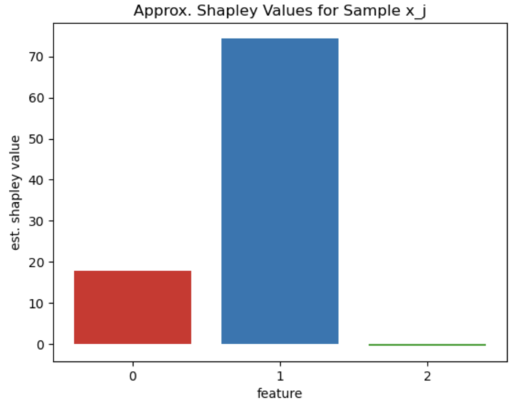
Figure 1: Shapley values for sample x_1
The results are illustrated in Figure 1. This demonstrates that for x_1, feature 1 provides the dominant contribution in this model. On the other hand, feature 2 has the lowest contribution by far.
All Samples Analysis
Let’s build upon the last subsection, to now compute Shapley Values for all the samples in our dataset X. Afterwards, we can plot the distribution of these values per feature, and also compare them with the coefficients from the linear regression model.
# compute shapley values for all samples
results = {0:[],1:[],2:[]}
for j in range(X.shape[0]):
    x_j = X[j,:]
    for i in range(X.shape[1]):
        results[i].append(approx_shapley(x_j, i, M, X, model))

# plot the distributions
plt.hist(results[0], alpha=0.5, bins=10, label='0')
plt.hist(results[1], alpha=0.5, bins=10, label='1')
plt.hist(results[2], alpha=0.5, bins=10, label='2')
plt.xlabel('shapley value')
plt.ylabel('count')
plt.title('Distribution of Shapley Values for all Features')
plt.legend(title='features')
plt.show()
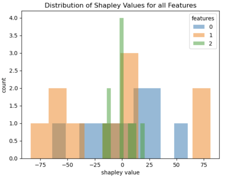
Figure 2: distribution of Shapley values for all data in X
The results visualized in Figure 2 show that feature 1 tends to have the largest absolute Shapley Values. Feature 0 produces values that are somewhat more compact around 0.0, while feature 2 yields Shapley values that lie the closest to zero. Therefore, these results indicate that feature 1 is the most important, followed by feature 0. Feature 2 is the least relevant to the problem at hand.
Since we normalized our data at the start of this analysis, the coefficients in our linear model should correspond to the conclusions above. We can check this out now:
model.fit(X,y)
model.coef_
array([33.17695477, 54.12190107, 11.73925815])
The magnitude of the coefficient reflects the relative importance of the feature. It is apparent that feature 1 has the largest coefficient, followed by feature 0, and then feature 2. This matches our expectations from the computed Shapley Values.
Final Remarks & Video
In this post you have learned:
- Why we need Shapley Values in machine learning
- Why the classic Shapley Value definition is not suitable for practical machine learning problems
- How Approximate Shapley Values can be computed that circumvent the problems with the classic definition
- How to implement the Approximate Shapley Value algorithm from scratch in Python
If you prefer video format, I also have a video where I cover the material presented here:
I hope you enjoyed this article, and gained some value from it. If you would like to take a closer look at the code presented here, please take a look at my GitHub. If you have any questions or suggestions, please feel free to add a comment below. Your input is greatly appreciated.
Note I have started a New Monthly Newsletter! At the end of each month I will send out this free newsletter to each of my subscribers by email. This is the best way to stay on top of my latest content. Sign up for the newsletter here!
Related Posts
Hi I'm Michael Attard, a Data Scientist with a background in Astrophysics. I enjoy helping others on their journey to learn more about machine learning, and how it can be applied in industry.
