Global Model Explainability refers to the ability to understand, and quantify, what drives decisions in a machine learning model across an entire dataset. This typicall implies an understanding of how the input predictor features influence the output of the model. In this post, we’ll experiment with 2 different approaches to this problem: summed SHAP values and SAGE. All code here is available on my Github.
Table of Contents

Testing 2 Techniques for Global Model Explainability – image by author
Video
For those who prefer video format, below you can watch me cover the contents of this article on YouTube:
Introduction to Global Model Explainability
Explainable AI (XAI) is growing trend within artificial intelligence and machine learning. For certain industries like finance and healthcare, it is critically important to be able to explain both:
- why models make the individual predictions that they do? (Local Explainability)
- how the model functions in a holistic sense? (Global Explainability)
A popular package for XAI is SHAP, however this library focuses on explainability for individual model predictions. This addresses point 1. above, but what are we to do for global explainability?
Global Model Explainability refers to understanding what drives the models decisions over an entire data generation process, not just an individual prediction. This translates to being able to quantify how the input predictor features are affecting the models predictions overall.
In this post, we’ll cover 2 different approaches for tackling global explainability. These will include:
- compute the aforementioned SHAP values for each sample in our dataset, and sum their magnitudes
- make use of Shapley Additive Global importance (SAGE) – an algorithm designed to handle the problem of global explainability
Formally, SHAP values \phi approximate the contribution of feature j to the prediction for a specific sample x, with respect to the models expected output. When we sum these values over all samples in a dataset we get:
\text{Global Importance}_j = \sum_x|\phi_j(x)|
This is a heuristic aggregation of local contributions, not a well-defined global metric. It answers a question like:
“On average, how much does feature j matter for individual predictions?”
SAGE was introduced to explicitly define a global Shapley framework for feature importance, derived from model performance degradation. It defines a value function v(S) that measures how well the model performs when only a subset of features S
is available.
For example, set v(S) = \text{Performance}(f_S), where f_S is our model with S features known. Then the SAGE value is simply the Shapley value for v:
\phi_j = E_{S \subseteq D\ \{j\} }[v(S \cup \{j\}) – v(S)]
where D is the total set of features available. SAGE answers the question: “How much does each feature contribute to the model’s predictive performance, averaged over all possible feature subsets?”
Experiment Setup
Our aim is to demonstrate some of the properties of the two aforementioned approaches to global explainability. To this end, we will work with a simple toy regression dataset that we will implement in Python. Furthermore, we will check how the explainability results different between two very different modeling algorithms: Linear Regression and Random Forest.
We can start by importing the required packages for this experiment:
# import
import numpy as np
import pandas as pd
from sklearn.ensemble import RandomForestRegressor
from sklearn.linear_model import LinearRegression
from sklearn.model_selection import train_test_split
from sklearn.metrics import mean_squared_error
import matplotlib.pyplot as plt
import shap
import sage
Let’s now setup a simple dataset involving 3 features (X1, X2, X3), two of which are informative (X1, X2). The dataset will consist of 10000 samples, and our target will have a linear relationship with X1 and X2. Finally, we’ll do a train-test split, leaving 20% of the data out for testing:
# simple dataset of 10000 samples
n_samples = 10000
random_state = 42
rng = np.random.RandomState(random_state)

X1 = rng.normal(0, 1, n_samples)
X2 = rng.normal(0, 1.5, n_samples)
X3 = rng.normal(0, 1, n_samples)
y = 1.5 * X1 + 2 * X2 + rng.normal(0, 0.5, n_samples)

X = np.vstack([X1, X2, X3]).T
feature_names = ["X1", "X2", "X3"]

X_train, X_test, y_train, y_test = train_test_split(X, y, test_size=0.2, random_state=random_state)
We can now visualize the data:
# visualize the results
plt.scatter(X1, y, label="X1", color="blue", alpha=0.3)
plt.scatter(X2, y, label="X2", color="orange", alpha=0.3)
plt.scatter(X3, y, label="X3", color="green", alpha=0.3)
plt.legend()
plt.xlabel('feature space')
plt.ylabel('y')
plt.title('3 Input Predictor Features')
plt.show()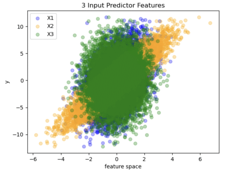
Figure 1: Distribution of data points generated in the toy dataset
The distribution of data points shown in Figure 1 illustrates the relative correlation between the target (y) and each of the individual features. Note that X3 is completely symmetric about x = 0, highlighting the fact that this feature is uninformative.
Build Models
As mentioned at the beginning, we’ll try out 2 algorithms for the modelling task. These will include the scikit-learn implementations of linear regression and random forest. For both we will keep all hyper parameters to their default values, except for setting the random state:
# declare and train model instances
rf = RandomForestRegressor(random_state=random_state)
lr = LinearRegression()
rf.fit(X_train, y_train)
lr.fit(X_train, y_train)

print("Linear Regression Test RMSE:", np.sqrt(mean_squared_error(y_test, lr.predict(X_test))))
print("Random Forest Test RMSE:", np.sqrt(mean_squared_error(y_test, rf.predict(X_test))))
Linear Regression Test RMSE: 0.5088308581798484 Random Forest Test RMSE: 0.553364515516271
We can see that the linear regression performs better on the test set, which should not be surprising given that the true underlying relationship is linear.
Explainability Logic
Now we can try out our 2 approaches for global explainability. To make things a bit more interesting, let’s modify the test set such that the sign for all the values for X2 are reversed. The consequence for this will be that this feature will drive the model towards making mistakes:
# reverse sign for X2 in test set
X_test[:,1] *= -1
%%time
# setup SHAP explainers
explainer = shap.Explainer(lr, X_train)
lr_shap_values = explainer(X_test)
explainer = shap.TreeExplainer(rf, X_train)
rf_shap_values = explainer(X_test)
# Aggregate to get global importances
shap_importance = np.mean(np.abs(lr_shap_values.values), axis=0)
lr_shap_rank = pd.Series(shap_importance, index=feature_names).sort_values(ascending=False)
shap_importance = np.mean(np.abs(rf_shap_values.values), axis=0)
rf_shap_rank = pd.Series(shap_importance, index=feature_names).sort_values(ascending=False)CPU times: user 21.9 s, sys: 55.2 ms, total: 22 s Wall time: 21.9 s
%%time

# compute SAGE values
imputer = sage.MarginalImputer(lr, X_test)
estimator = sage.PermutationEstimator(imputer, 'mse')
lr_sage_values = estimator(X_test, y_test)
imputer = sage.MarginalImputer(rf, X_test)
estimator = sage.PermutationEstimator(imputer, 'mse')
rf_sage_values = estimator(X_test, y_test)

# rank the features based on their sage values
lr_sage_rank = pd.Series(lr_sage_values.values, index=feature_names).sort_values(ascending=False)
rf_sage_rank = pd.Series(rf_sage_values.values, index=feature_names).sort_values(ascending=False)
CPU times: user 1min 22s, sys: 756 ms, total: 1min 23s Wall time: 1min 23s
# compare linear regression results
lr_comparison = pd.DataFrame({
    "SHAP_importance": lr_shap_rank,
    "SAGE_importance": lr_sage_rank
})
print(f"\nComparison of feature rankings for linear regression:\n\n{lr_comparison}")
Comparison of feature rankings for linear regression:
SHAP_importance SAGE_importance
X1 1.213376 2.260730
X2 2.391002 -26.974467
X3 0.001451 0.000812 # compare random forest results
rf_comparison = pd.DataFrame({
"SHAP_importance": rf_shap_rank,
"SAGE_importance": rf_sage_rank
})
print(f"\nComparison of feature rankings for random forest:\n\n{rf_comparison}")Comparison of feature rankings for random forest:
SHAP_importance SAGE_importance
X1 1.196237 1.923315
X2 2.380982 -26.845748
X3 0.029678 -0.001912 Final Remarks
We can note the following conclusions from these tests:
- The importances are largely consistent regardless of the choice of model (linear regression or random forest)
- Both methods correctly capture that X1 and X2 are informative features, and X3 is not
- The aggregated SHAP values cannot indicate whether a feature tends to drive the model towards better performance or not. It simply shows that X2 is influential, and that is all. In contrast, SAGE shows that X2 drives the model towards making mistakes, as seen by the large negative value assigned to this feature
- The downside of SAGE is that it is computationally expensive: it took about 4 times longer to run SAGE than the aggregated SHAP approach
I hope you enjoyed this article, and gained some value from it. If you would like to take a closer look at the code presented here, please take a look at my GitHub. If you have any questions or suggestions, please feel free to add a comment below. Your input is greatly appreciated.
Interested in signing up for my Monthly Newsletter? At the end of each month I will send out this free newsletter to each of my subscribers by email. This is the best way to stay on top of my latest content. Sign up for the newsletter here!
Related Posts
Hi I'm Michael Attard, a Data Scientist with a background in Astrophysics. I enjoy helping others on their journey to learn more about machine learning, and how it can be applied in industry.