Learning from Positive and Unlabeled Data: PU Bagging + XGBoost on 20 Newsgroups

Positive and Unlabeled data is a common occurrence in a variety of industries, ranging from healthcare, to recommendation systems, and fraud detection to name a few. In this post, we’ll explore one technique for handling such a scenario, PU Bagging, on the 20 Newsgroup dataset. All coding examples shown below are done in Python, and available on my Github.

Table of Contents

Learning from Positive and Unlabeled Data – image by author

What are Positive Unlabeled data?

Positive Unlabeled (PU) data comprise a dataset that contains a set of confirmed positive examples, and a much larger pool of unlabeled samples. As such, the unlabeled pool contains samples that could either be positive or negative. Therefore it is a mixture of negatives and hidden positives that simply haven’t been labeled.

This situation arises whenever confirming a label is difficult, expensive, or effectively impossible. Specific cases could include a diagnosed disease case, a completed purchase, a confirmed fraud, a species sighting, etc.

What is PU Bagging?

PU learning is the branch of machine learning dedicated to building useful classifiers from exactly this kind of asymmetric, incomplete labeling. PU Bagging (the method covered in this post) is one of the more practical and widely used approaches for accomplishing this task. PU Bagging was originally developed by Mordelet, F. and Vert J.P. 2010, and we will be examining the inductive algorithm (Algorithm 1) from that paper.

PU Bagging revolves around training a series of $T$ classifiers on data constructed as follows:

draw a bootstrapped sample with replacement from the unlabeled population (called $U$ )
combine the bootstrapped sample with the known positive samples (called $P$ )
train the $t^{\text(th)}$ classifier to distinguish between $U$ and $P$
repeat the above steps for $t = 1\dotsT$

The output from the trained classifiers can then be combined to yield a net prediction on unseen data. Formally we can define the algorithm as:

$\text{for} \; t = 1 \; \text{to} \; T \text{:}$
$\quad \text{Draw a sample} \; U_t \; \text{of size} \; K \; \text{from} \; U_t$
$\quad \text{Train a classifier} \; f_t \; \text{to discriminate} \; P \; \text{from} \; U_t$
Compute: $f = \frac{1}{T}\sum_{t=1}^Tf_t$

An illustration of this procedure is presented below:

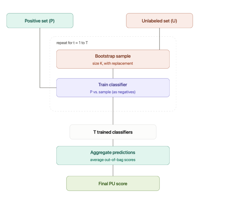
Figure 1: flowchart depiction of Algorithm 1 from Mordelet and Vert 2010

Setup the Python Environment

We will be making use of the 20 Newsgroups dataset, that consists of twenty distinct categories of news articles. For modeling, I will use the popular XGBoost Classifier.

Let’s start by importing the packages needed for our experiment:

import numpy as np
import matplotlib.pyplot as plt
from xgboost import XGBClassifier
from sklearn.datasets import fetch_20newsgroups
from sklearn.feature_extraction.text import TfidfVectorizer
from sklearn.model_selection import train_test_split
from sklearn.base import clone
from sklearn.metrics import (
    auc, 
    precision_recall_curve,
    precision_score, 
    recall_score, 
    f1_score
)

We can now load in the data, and plot the frequency of the different categories in both our training and test data sets:

# load data
data_train = fetch_20newsgroups(subset="train")
data_test = fetch_20newsgroups(subset="test")

X_train = data_train.data
y_train = data_train.target
X_test = data_test.data
y_test = data_test.target
target_names = data_train.target_names

# function to plot frequencies
def plot_label_frequency(y, target_names, title):
    labels, counts = np.unique(y, return_counts=True)
    class_names = [target_names[i] for i in labels]

    plt.figure(figsize=(12, 6))
    plt.bar(class_names, counts)
    plt.xlabel("Newsgroup")
    plt.ylabel("Frequency")
    plt.title(title)
    plt.xticks(rotation=45)
    plt.tight_layout()
    plt.show()
    
# plot frequencies of training data
plot_label_frequency(y_train, target_names, "Frequency of Classes in 20 Newsgroups Training Dataset")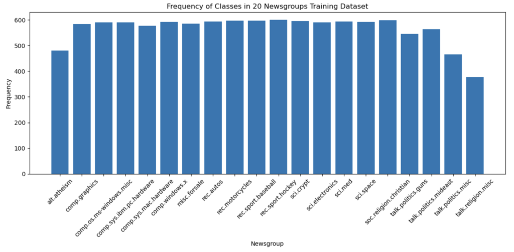

# plot frequencies of test data
plot_label_frequency(y_test, target_names, "Frequency of Classes in 20 Newsgroups Testing Dataset")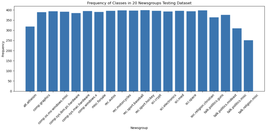

We can see that the majority of the classes in our training data have a frequency of just under ~600, whereas in the test data these same categories have a frequency around ~400. Note that certain topics, like atheism, religion, and politics, have significantly lower frequencies.

We can now move on to preprocessing our data. This will involve converting our text into TF-IDF features, by making use of TfidfVectorizer from scikit-learn. I will also remove English stop words by making use of the built-in stop word list, and I will create features for 1 ngrams:

preprocessor = TfidfVectorizer(stop_words='english', ngram_range=(1,1))
X_train = preprocessor.fit_transform(X_train)
X_test = preprocessor.transform(X_test)
print(f"Number of training samples: {X_train.shape[0]}, number of test samples: {X_test.shape[0]}, number of features created: {X_train.shape[1]}")

Number of training samples: 11314, number of test samples: 7532, number of features created: 129796

Just over one hundred thousand features have been created through our procedure. This is substantially larger than the number of samples we have in the data, therefore care will be needed to adequately regularize our classifier. I will do this primarily by limiting the amount by which each tree in the XGBoost classifier can grow.

Let’s now define our model:

model = XGBClassifier(n_estimators=50, max_depth=3, random_state=42, n_jobs=-1)
threshold = 0.5

Our XGBoost classifier will consist of 50 trees, each of which will be permitted a max_depth of 3. Note I have also set our cutoff threshold to be 0.5 for this experiment.

Lastly, I’ll define a few helper functions for the coming sections:

def split_idx(y_labels, label) -> tuple:
    positive_idx = np.where(y_labels == label)[0]
    other_idx = np.where(y_labels != label)[0]
    return(positive_idx, other_idx)

def assemble_labels(pos_idx, oth_idx, y_in) -> np.array:
    # create copy
    y = np.copy(y_in)

    # assign label values
    y[pos_idx] = 1
    y[oth_idx] = 0

    return y

def generate_indices(y, g, ratio_hidden_pos) -> tuple:
    # obtain indices for label g
    pos_idx, oth_idx = split_idx(y, g)

    # randomly select some positives to be hidden in the training data
    pos_idx, hidden_pos_idx = train_test_split(
        pos_idx,
        test_size=ratio_hidden_pos,
        random_state=42
    )

    # construct the unlabeled index set:
    #   - all genuinely negative examples
    #   - the hidden positive examples
    unlabeled_idx = np.concatenate([
        oth_idx,
        hidden_pos_idx
    ])

    return(pos_idx, unlabeled_idx)

Baseline 1 - Completely Labeled Dataset

A first point of comparison is to evaluate how well our model does on a completely labeled dataset – this should represent an upper bound on overall performance that we can expect. In this situation, there is no ambiguity over the labels:

mean_auc, mean_p, mean_r, mean_f = [], [], [], []
# iterate through each label in the data
for g in np.unique(y_train):
    # obtain indices for label g in train set
    pos_train_idx, oth_train_idx = split_idx(y_train, g)

    # set labels equal to g to be 1, otherwise 0
    y_train_g = assemble_labels(pos_train_idx, oth_train_idx, y_train)
    
    # obtain indices for label g in test set
    pos_test_idx, oth_test_idx = split_idx(y_test, g)

    # set labels equal to g to be 1, otherwise 0  
    y_test_g = assemble_labels(pos_test_idx, oth_test_idx, y_test)
    
    # train the model
    model.fit(X_train, y_train_g)

    # evaluate
    y_proba = model.predict_proba(X_test)[:,1]
    y_pred = (y_proba > threshold).astype(int)
    precision, recall, _ = precision_recall_curve(y_test_g, y_proba)
    prauc = auc(recall, precision)
    #auc = roc_auc_score(y_test_g, y_proba)
    p = precision_score(y_test_g, y_pred, pos_label=1)
    r = recall_score(y_test_g, y_pred, pos_label=1)
    f = f1_score(y_test_g, y_pred, pos_label=1)
    print(f"Class {g}:\nPR AUC = {prauc:.2f}, Precision = {p:.2f}, Recall = {r:.2f}, F1 = {f:.2f}")

    # record results
    mean_auc.append(prauc) 
    mean_p.append(p)
    mean_r.append(r)
    mean_f.append(f)

# print mean results
mean_auc = np.mean(mean_auc)
mean_p = np.mean(mean_p)
mean_r = np.mean(mean_r)
mean_f = np.mean(mean_f)
print(f"\nMean PR AUC: {mean_auc:.2f}, Mean Precision: {mean_p:.2f}, Mean Recall: {mean_r:.2f}, Mean F1: {mean_f:.2f}")

Class 0:
PR AUC = 0.74, Precision = 0.80, Recall = 0.52, F1 = 0.63
Class 1:
PR AUC = 0.63, Precision = 0.74, Recall = 0.46, F1 = 0.56
Class 2:
PR AUC = 0.71, Precision = 0.77, Recall = 0.55, F1 = 0.64
Class 3:
PR AUC = 0.57, Precision = 0.73, Recall = 0.39, F1 = 0.51
Class 4:
PR AUC = 0.79, Precision = 0.84, Recall = 0.60, F1 = 0.70
Class 5:
PR AUC = 0.77, Precision = 0.90, Recall = 0.54, F1 = 0.68
Class 6:
PR AUC = 0.85, Precision = 0.87, Recall = 0.72, F1 = 0.78
Class 7:
PR AUC = 0.78, Precision = 0.88, Recall = 0.60, F1 = 0.71
Class 8:
PR AUC = 0.89, Precision = 0.93, Recall = 0.77, F1 = 0.85
Class 9:
PR AUC = 0.86, Precision = 0.94, Recall = 0.61, F1 = 0.74
Class 10:
PR AUC = 0.94, Precision = 0.96, Recall = 0.79, F1 = 0.87
Class 11:
PR AUC = 0.91, Precision = 0.94, Recall = 0.79, F1 = 0.86
Class 12:
PR AUC = 0.50, Precision = 0.79, Recall = 0.23, F1 = 0.36
Class 13:
PR AUC = 0.74, Precision = 0.92, Recall = 0.41, F1 = 0.56
Class 14:
PR AUC = 0.89, Precision = 0.94, Recall = 0.70, F1 = 0.80
Class 15:
PR AUC = 0.91, Precision = 0.91, Recall = 0.72, F1 = 0.81
Class 16:
PR AUC = 0.73, Precision = 0.73, Recall = 0.68, F1 = 0.70
Class 17:
PR AUC = 0.87, Precision = 0.98, Recall = 0.64, F1 = 0.78
Class 18:
PR AUC = 0.64, Precision = 0.85, Recall = 0.39, F1 = 0.53
Class 19:
PR AUC = 0.44, Precision = 0.59, Recall = 0.26, F1 = 0.36

Mean PR AUC: 0.76, Mean Precision: 0.85, Mean Recall: 0.57, Mean F1: 0.67

Here we can see the model performance per class, as well as the mean results over all classes.

Baseline 2 - Naive Approach to PU Data

Let’s now setup the PU-learning scenario. For each newsgroup $g$ , we need to extract out a sample from all rows labelled $g$ and keep the remaining rows as unlabelled. Then during training, we can take the naive approach and label all unlabelled rows to be negative (0).

positive_labelled = 0.7

mean_auc, mean_p, mean_r, mean_f = [], [], [], []
# iterate through each label in the data
for g in np.unique(y_train):
    # generate indices for PU training dataset
    pos_train_idx, unlabeled_train_idx = generate_indices(y_train, g, 1.0-positive_labelled)

    # create the training labels
    y_train_g = assemble_labels(pos_train_idx, unlabeled_train_idx, y_train)

    # obtain indices for label g in test set
    pos_test_idx, oth_test_idx = split_idx(y_test, g)

    # set test labels equal to g to be 1, otherwise 0  
    y_test_g = assemble_labels(pos_test_idx, oth_test_idx, y_test)
    
    # train the model
    model.fit(X_train, y_train_g)

    # evaluate
    y_proba = model.predict_proba(X_test)[:,1]
    y_pred = (y_proba > threshold).astype(int)
    #auc = roc_auc_score(y_test_g, y_proba)
    precision, recall, _ = precision_recall_curve(y_test_g, y_proba)
    prauc = auc(recall, precision)
    p = precision_score(y_test_g, y_pred, pos_label=1)
    r = recall_score(y_test_g, y_pred, pos_label=1)
    f = f1_score(y_test_g, y_pred, pos_label=1)
    print(f"Class {g}:\nPR AUC = {prauc:.2f}, Precision = {p:.2f}, Recall = {r:.2f}, F1 = {f:.2f}")

    # record results
    mean_auc.append(prauc) 
    mean_p.append(p)
    mean_r.append(r)
    mean_f.append(f)

# print mean results
mean_auc = np.mean(mean_auc)
mean_p = np.mean(mean_p)
mean_r = np.mean(mean_r)
mean_f = np.mean(mean_f)
print(f"\nMean PR AUC: {mean_auc:.2f}, Mean Precision: {mean_p:.2f}, Mean Recall: {mean_r:.2f}, Mean F1: {mean_f:.2f}")

Class 0:
PR AUC = 0.64, Precision = 0.83, Recall = 0.28, F1 = 0.41
Class 1:
PR AUC = 0.58, Precision = 0.78, Recall = 0.29, F1 = 0.42
Class 2:
PR AUC = 0.69, Precision = 0.84, Recall = 0.30, F1 = 0.44
Class 3:
PR AUC = 0.51, Precision = 0.79, Recall = 0.21, F1 = 0.34
Class 4:
PR AUC = 0.71, Precision = 0.87, Recall = 0.39, F1 = 0.54
Class 5:
PR AUC = 0.72, Precision = 0.92, Recall = 0.36, F1 = 0.52
Class 6:
PR AUC = 0.78, Precision = 0.88, Recall = 0.52, F1 = 0.65
Class 7:
PR AUC = 0.74, Precision = 0.93, Recall = 0.35, F1 = 0.51
Class 8:
PR AUC = 0.87, Precision = 0.95, Recall = 0.58, F1 = 0.72
Class 9:
PR AUC = 0.75, Precision = 0.91, Recall = 0.32, F1 = 0.48
Class 10:
PR AUC = 0.89, Precision = 0.97, Recall = 0.56, F1 = 0.71
Class 11:
PR AUC = 0.85, Precision = 0.97, Recall = 0.52, F1 = 0.67
Class 12:
PR AUC = 0.49, Precision = 0.86, Recall = 0.17, F1 = 0.28
Class 13:
PR AUC = 0.69, Precision = 0.98, Recall = 0.23, F1 = 0.37
Class 14:
PR AUC = 0.81, Precision = 0.98, Recall = 0.46, F1 = 0.63
Class 15:
PR AUC = 0.85, Precision = 0.94, Recall = 0.50, F1 = 0.65
Class 16:
PR AUC = 0.65, Precision = 0.73, Recall = 0.48, F1 = 0.58
Class 17:
PR AUC = 0.80, Precision = 0.98, Recall = 0.43, F1 = 0.60
Class 18:
PR AUC = 0.55, Precision = 0.90, Recall = 0.26, F1 = 0.41
Class 19:
PR AUC = 0.41, Precision = 0.58, Recall = 0.16, F1 = 0.25

Mean PR AUC: 0.70, Mean Precision: 0.88, Mean Recall: 0.37, Mean F1: 0.51

The PR AUC drops a bit in comparision with what we saw with Baseline 1, while Precision improved at bit, but Recall has significantly declined (and the F1 score along with it). This indicates that the model struggles more to capture all positive cases in the test set, now that 30% of the positive labels are treated as negatives in the training data.

Let’s now compute results using the PU Bagging method, and compare the results we the two baselines we can just obtained.

PU Bagging

Now let’s try out the PU Bagging algorithm defined earlier. Here we’ll be using 10 bags, where each includes a total of 600 samples. We’ll be assigning the same percentage of positive cases to the unlabeled category as was done for Baseline 2:

# set bootstrap parameters
T = 10
K = 600

mean_auc, mean_p, mean_r, mean_f = [], [], [], []
# iterate through each label in the data
for g in np.unique(y_train):

    ### SETUP PU TRAINING DATA ###

    # generate indices for PU training dataset
    pos_train_idx, unlabeled_train_idx = generate_indices(y_train, g, 1.0-positive_labelled)

    # loop over all bootstrap samples
    ensemble = []
    for t in range(T):
        # extract data for boostrap t
        u_idx = np.random.choice(unlabeled_train_idx, size=K, replace=True)
        U_y = np.zeros(u_idx.shape[0])
        P_y = np.ones(pos_train_idx.shape[0])

        # prepare data for training
        x_idx = np.concatenate([u_idx, pos_train_idx])
        X = X_train[x_idx]
        y = np.concatenate([U_y, P_y])

        # train model and store
        model_t = clone(model)
        model_t.fit(X, y)
        ensemble.append(model_t)
    
    ### SETUP TEST DATA ###

    # obtain indices for label g in test set
    pos_test_idx, oth_test_idx = split_idx(y_test, g)

    # set test labels equal to g to be 1, otherwise 0  
    y_test_g = assemble_labels(pos_test_idx, oth_test_idx, y_test)

    ### GENERATE PREDICTIONS & EVALUATE ###
    
    # generate ensemble predictions
    y_proba = 0.0
    for model in ensemble:
        y_proba += model.predict_proba(X_test)[:,1]
    y_proba /= T
    y_pred = (y_proba > threshold).astype(int)
    
    # evaluate
    precision, recall, _ = precision_recall_curve(y_test_g, y_proba)
    prauc = auc(recall, precision)
    p = precision_score(y_test_g, y_pred, pos_label=1)
    r = recall_score(y_test_g, y_pred, pos_label=1)
    f = f1_score(y_test_g, y_pred, pos_label=1)
    print(f"Class {g}:\nPR AUC = {prauc:.2f}, Precision = {p:.2f}, Recall = {r:.2f}, F1 = {f:.2f}")

    # record results
    mean_auc.append(prauc) 
    mean_p.append(p)
    mean_r.append(r)
    mean_f.append(f)

# print mean results
mean_auc = np.mean(mean_auc)
mean_p = np.mean(mean_p)
mean_r = np.mean(mean_r)
mean_f = np.mean(mean_f)
print(f"\nMean PR AUC: {mean_auc:.2f}, Mean Precision: {mean_p:.2f}, Mean Recall: {mean_r:.2f}, Mean F1: {mean_f:.2f}")

Class 0:
PR AUC = 0.61, Precision = 0.51, Recall = 0.69, F1 = 0.59
Class 1:
PR AUC = 0.60, Precision = 0.39, Recall = 0.73, F1 = 0.51
Class 2:
PR AUC = 0.66, Precision = 0.49, Recall = 0.78, F1 = 0.60
Class 3:
PR AUC = 0.52, Precision = 0.34, Recall = 0.77, F1 = 0.47
Class 4:
PR AUC = 0.70, Precision = 0.50, Recall = 0.80, F1 = 0.61
Class 5:
PR AUC = 0.71, Precision = 0.59, Recall = 0.75, F1 = 0.66
Class 6:
PR AUC = 0.82, Precision = 0.69, Recall = 0.89, F1 = 0.78
Class 7:
PR AUC = 0.71, Precision = 0.65, Recall = 0.73, F1 = 0.69
Class 8:
PR AUC = 0.88, Precision = 0.83, Recall = 0.83, F1 = 0.83
Class 9:
PR AUC = 0.74, Precision = 0.54, Recall = 0.81, F1 = 0.64
Class 10:
PR AUC = 0.91, Precision = 0.78, Recall = 0.88, F1 = 0.83
Class 11:
PR AUC = 0.85, Precision = 0.79, Recall = 0.80, F1 = 0.79
Class 12:
PR AUC = 0.44, Precision = 0.33, Recall = 0.53, F1 = 0.41
Class 13:
PR AUC = 0.71, Precision = 0.67, Recall = 0.65, F1 = 0.66
Class 14:
PR AUC = 0.82, Precision = 0.69, Recall = 0.77, F1 = 0.73
Class 15:
PR AUC = 0.86, Precision = 0.67, Recall = 0.90, F1 = 0.77
Class 16:
PR AUC = 0.68, Precision = 0.54, Recall = 0.82, F1 = 0.65
Class 17:
PR AUC = 0.82, Precision = 0.89, Recall = 0.70, F1 = 0.78
Class 18:
PR AUC = 0.51, Precision = 0.40, Recall = 0.65, F1 = 0.49
Class 19:
PR AUC = 0.27, Precision = 0.26, Recall = 0.57, F1 = 0.35

Mean PR AUC: 0.69, Mean Precision: 0.58, Mean Recall: 0.75, Mean F1: 0.64

Final Remarks

Let’s tabulate the results we have obtained:

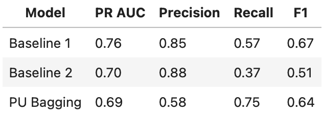
For the specific configuration tested here (threshold equal to 0.5, 10 bags, bag size of 600), we can see that the main advantage of PU Bagging comes in terms of Recall. In other words, PU Bagging is shown to provide the best means by which to find all positive values in the test set. This comes at the expense of Precision, indicating that the the PU Bagging approach does yield more False Positives compared to the baselines.

A more thorough analysis would experiment with trying different values for the following parameters:

classifier threshold
number of PU bags
size of PU bags
percentage of positives included in the unlabelled dataset
hyperparameters of the XGBoost model

Diving into this is beyond the scope of this notebook. Feel free to try it out yourself!

I hope you enjoyed this article, and gained some value from it. If you would like to take a closer look at the code presented here, please take a look at my GitHub. If you have any questions or suggestions, please feel free to add a comment below. Your input is greatly appreciated.

Interested in signing up for my Monthly Newsletter? At the end of each month I will send out this free newsletter to each of my subscribers by email. This is the best way to stay on top of my latest content. Sign up for the newsletter here!

Hi I'm Michael Attard, a Data Scientist with a background in Astrophysics. I enjoy helping others on their journey to learn more about machine learning, and how it can be applied in industry.

Cookie	Duration	Description
cookielawinfo-checkbox-analytics	11 months	This cookie is set by GDPR Cookie Consent plugin. The cookie is used to store the user consent for the cookies in the category "Analytics".
cookielawinfo-checkbox-functional	11 months	The cookie is set by GDPR cookie consent to record the user consent for the cookies in the category "Functional".
cookielawinfo-checkbox-necessary	11 months	This cookie is set by GDPR Cookie Consent plugin. The cookies is used to store the user consent for the cookies in the category "Necessary".
cookielawinfo-checkbox-others	11 months	This cookie is set by GDPR Cookie Consent plugin. The cookie is used to store the user consent for the cookies in the category "Other.
cookielawinfo-checkbox-performance	11 months	This cookie is set by GDPR Cookie Consent plugin. The cookie is used to store the user consent for the cookies in the category "Performance".
viewed_cookie_policy	11 months	The cookie is set by the GDPR Cookie Consent plugin and is used to store whether or not user has consented to the use of cookies. It does not store any personal data.